Fluid Simulation in 200 Lines of Code

4 minute(s) de lecture

Have you ever wondered how realistic fluid simulations in movies or games are created? It might seem like black magic involving complex physics and heavy computation, but the core concepts are surprisingly accessible.

In his “Ten Minute Physics” series, Matthias Müller demonstrates how to write an Eulerian fluid simulator in just about 200 lines of JavaScript. Based on his video Ten Minute Physics 17 and the accompanying paper, this post breaks down the magic behind computational fluid dynamics (CFD).

The Physics: Navier-Stokes Equations

At the heart of fluid simulation are the Navier-Stokes equations. For an incompressible fluid (like water), they look like this:

\[\frac{\partial \mathbf{u}}{\partial t} + (\mathbf{u} \cdot \nabla) \mathbf{u} = -\frac{1}{\rho} \nabla p + \nu \nabla^2 \mathbf{u} + \mathbf{f}\] \[\nabla \cdot \mathbf{u} = 0\]

Where:

$\mathbf{u}$ is the velocity field.
$\rho$ is the density.
$p$ is the pressure.
$\nu$ is the kinematic viscosity.
$\mathbf{f}$ represents external forces (like gravity).

The first equation describes how the velocity changes over time due to advection, pressure, viscosity, and external forces. The second equation enforces incompressibility, meaning the amount of fluid flowing into any region must equal the amount flowing out.

The Two Perspectives: Lagrangian vs. Eulerian

When simulating fluids, there are two main approaches:

Lagrangian (Particle-based): You treat the fluid as a collection of particles and track each one’s position and velocity. This is intuitive, like simulating a bunch of marbles. Smoothed Particle Hydrodynamics (SPH) is a popular example.
Eulerian (Grid-based): You divide the space into a fixed grid. Instead of tracking particles, you track the fluid properties (like velocity and density) at each grid cell. It’s like measuring the wind speed at fixed weather stations.

For this simulation, we use the Eulerian approach because it’s often easier to handle incompressibility and produces smooth results for things like smoke.

The Staggered Grid

A key trick in Eulerian simulation is using a staggered grid. Instead of storing all variables (pressure, horizontal velocity $u$, vertical velocity $v$) at the center of each cell, we offset them:

Pressure ($p$): Stored at the cell center $(i, j)$.
Horizontal Velocity ($u$): Stored at the center of the vertical cell faces $(i+1/2, j)$.
Vertical Velocity ($v$): Stored at the center of the horizontal cell faces $(i, j+1/2)$.

Staggered Grid Diagram
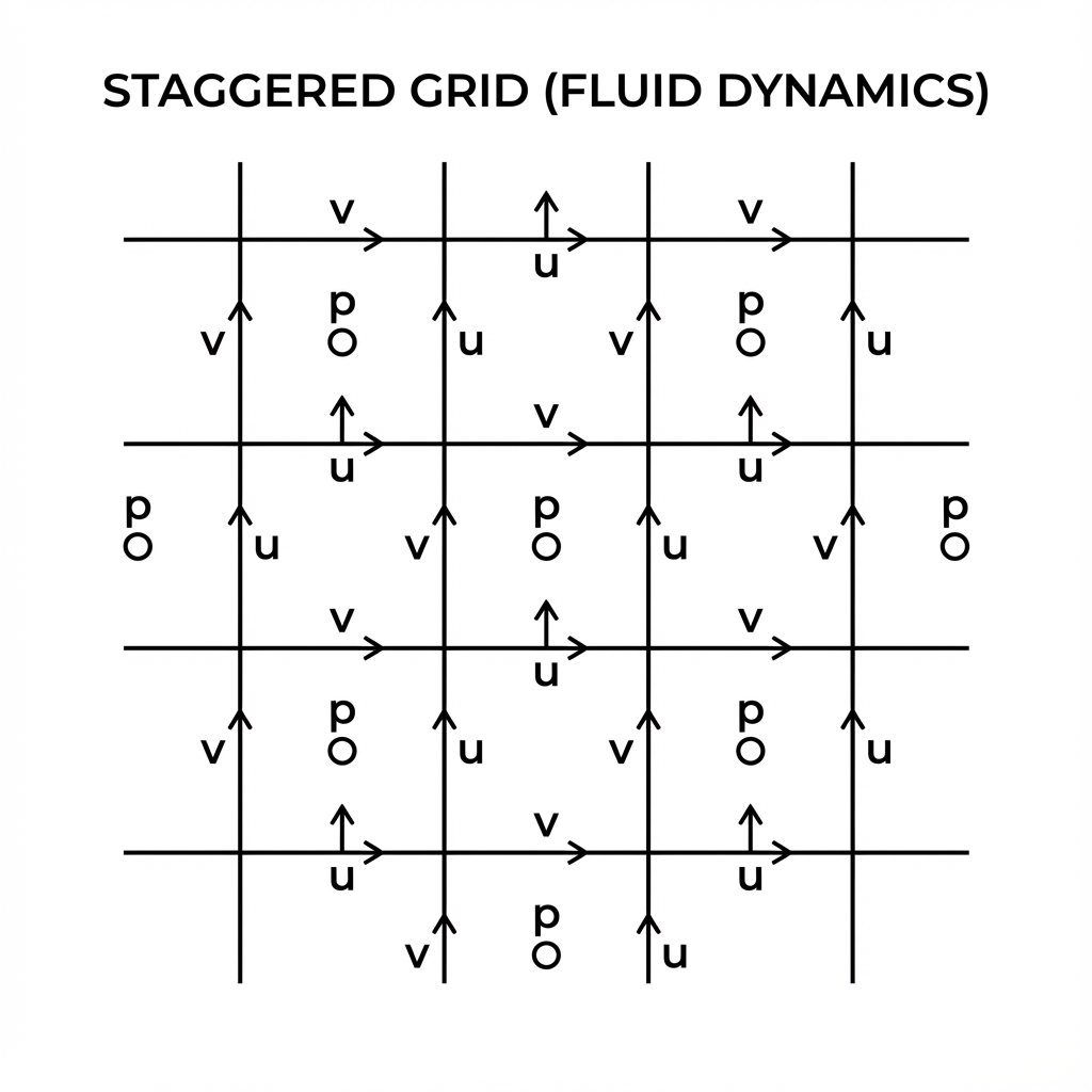
The Staggered Grid Arrangement

This arrangement prevents numerical instabilities (like the “checkerboard problem”) and makes calculating gradients and divergence much more accurate. For example, the derivative $\frac{\partial p}{\partial x}$ is naturally defined at the location of $u$.

The Algorithm

We solve the equations using operator splitting, which means we handle each term of the Navier-Stokes equation sequentially. The simulation loop consists of three main steps, repeated every frame:

External Forces: $\mathbf{u} \leftarrow \mathbf{u} + \mathbf{f} \Delta t$
Projection (Incompressibility): Solve $\nabla \cdot \mathbf{u} = 0$ by adjusting pressure.
Advection: Move the fluid (and the velocity field itself) along the flow.

1. External Forces

This is the simplest part. We just add gravity to the vertical velocity component.

integrate(dt, gravity) {
    var n = this.numY;
    for (var i = 1; i < this.numX; i++) {
        for (var j = 1; j < this.numY-1; j++) {
            if (this.s[i*n + j] != 0.0 && this.s[i*n + j-1] != 0.0)
                this.v[i*n + j] += gravity * dt;
        }
    }
}

2. Projection (Making it Incompressible)

Real fluids like water are incompressible—you can’t squeeze them into a smaller volume. In a grid, this means the amount of fluid entering a cell must equal the amount leaving it. Mathematically, the divergence of the velocity field must be zero ($\nabla \cdot \mathbf{u} = 0$).

If a cell has a net inflow (positive divergence), the pressure rises, pushing fluid out. We solve the Poisson equation for pressure:

\[\nabla^2 p = \frac{\rho}{\Delta t} \nabla \cdot \mathbf{u}\]

Once we have the pressure, we update the velocities to cancel out the divergence:

\[\mathbf{u}_{new} = \mathbf{u} - \frac{\Delta t}{\rho} \nabla p\]

We use an iterative method called Gauss-Seidel with Over-Relaxation (SOR) to speed up convergence.

solveIncompressibility(numIters, dt) {
    // ... setup ...
    for (var iter = 0; iter < numIters; iter++) {
        for (var i = 1; i < this.numX-1; i++) {
            for (var j = 1; j < this.numY-1; j++) {
                // ... check boundaries ...

                // Calculate divergence (net outflow)
                var div = this.u[(i+1)*n + j] - this.u[i*n + j] +
                          this.v[i*n + j+1] - this.v[i*n + j];

                // Calculate pressure correction
                var p = -div / s;
                p *= scene.overRelaxation; // SOR for speed
                this.p[i*n + j] += cp * p;

                // Update velocities
                this.u[i*n + j] -= sx0 * p;
                this.u[(i+1)*n + j] += sx1 * p;
                this.v[i*n + j] -= sy0 * p;
                this.v[i*n + j+1] += sy1 * p;
            }
        }
    }
}

3. Advection

Advection is the process of transporting quantities (like smoke density or temperature) along with the fluid flow. Crucially, the velocity field also advects itself!

We use a Semi-Lagrangian scheme. To find the new value of a quantity $q$ at a grid point $\mathbf{x}$, we trace the velocity vector backwards in time to find where the fluid particle came from ($\mathbf{x}_{prev}$), and sample the value at that previous position.

\[\mathbf{x}_{prev} = \mathbf{x} - \mathbf{u}(\mathbf{x}) \Delta t\] \[q_{new}(\mathbf{x}) = q_{old}(\mathbf{x}_{prev})\]

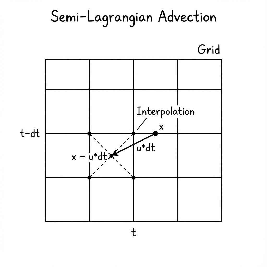
Semi-Lagrangian Advection Scheme

advectVel(dt) {
    this.newU.set(this.u);
    this.newV.set(this.v);

    // ... loop over grid ...
        // Trace back position: x_prev = x - u * dt
        var x = i*h;
        var y = j*h + h2;
        var u = this.u[i*n + j];
        var v = this.avgV(i, j);
        x = x - dt*u;
        y = y - dt*v;

        // Sample value at previous position
        u = this.sampleField(x,y, U_FIELD);
        this.newU[i*n + j] = u;
    // ... end loop ...

    this.u.set(this.newU);
    this.v.set(this.newV);
}

Conclusion

With just these three steps—Forces, Projection, and Advection—you can create a surprisingly realistic fluid simulation. The code is compact, efficient, and runs directly in the browser.

This implementation is a great starting point. From here, you can add obstacles, viscosity, different boundary conditions, or even extend it to 3D!

Check out the full source code and demo here.

Julien Guégan