
Kalman: filter, tracking, IMU
The Kalman filter is a very widespread method in the engineering field since it has numerous applications in localization, navigation, automatic piloting, object tracking, data fusion, etc. It was introduced in 1960 by the engineer Rudolf E. Kálmán and was notably used for trajectory estimation for the Apollo program. Indeed, from a series of measurements observed over time (noisy and biased), it makes it possible to calculate an estimate of these unknown variables that is often more precise than the measurements based on the theories of control and statistics. One of the strengths of this filter is its ability to improve over time by integrating an error term from the model itself. It has many other advantages: merging measurements from different sensors, working online, easy to implement…
Principle
The construction of the Kalman filter is based on 3 important assumptions:
- the modeled system is linear: it can be modeled as a multiplication between the state $t$ and $t-1$.
- the measurement noise is white: it is not correlated with time.
- the noise is Gaussian: it is described by an average and a covariance
The idea is to build a model for the state of the system that maximizes the posterior probability of these previous measurements. This means that the new model we build after making a measurement (taking into account both our previous model with its uncertainty and the new measurement with its uncertainty) is the model that has the highest probability of being correct . Furthermore, we can maximize the a posteriori probability without keeping a long history of the previous measurements themselves. Instead, we iteratively update the model of the system state and keep only this model for the next iteration. This greatly simplifies the computational implication of this method.
Static one-dimensional case
Suppose we want to know where to position a fixed point on a line and that we have 2 noisy measurements $x_1$ and $x_2$. Each of these measurements follows a Gaussian distribution:
\[p_i(x) = \frac{1}{\sigma_i\sqrt{2\pi}} e^{-\frac{(x-\bar{x}_i)^2}{2\sigma_i^2} } \quad (i=1,2)\]We can then show that the combination of these 2 Gaussian measurements is equivalent to a single Gaussian measurement characterized by the mean $\bar{x}_{12}$ and the variance $\sigma_{12}^2$:
\[\begin{aligned} \bar{x}_{12} &= \left( \frac{\sigma_2^2}{\sigma_1^2+\sigma_2^2} \right)x_1 + \left( \frac{ \sigma_1^2}{ \sigma_1^2+\sigma_2^2} \right)x_2 \\ \\ \sigma_{12}^2 &= \frac{\sigma_1^2\sigma_2^2}{\sigma_1^2+\sigma_2^2} \end{aligned}\]Thus, the new average value $\bar{x}_{12}$ is only a weighted combination of the two measurements by the relative uncertainties. For example, if the uncertainty $\sigma_2$ is particularly larger than $\sigma_1$, then the new average will be very close to $x_1$ which is more certain.
Now, if we start from the principle that we carry out our 2 measurements one after the other and that we therefore seek to estimate the current state of our system $(\hat{x}_t,\hat{\sigma}_t)$. At time $t=1$, we have our first measurement $\hat{x}_1=x_1$ and its uncertainty $\hat{\sigma}_1^2=\sigma_1^2$. Substituting this into our optimal estimating equations and rearranging them to separate the old information from the new information, we obtain:
\[\begin{aligned} \hat{x}_2 &= \hat{x}_1 + \frac{\hat\sigma_1^2}{\hat \sigma_1^2+\sigma_2^2}(x_2 - \hat x_1 ) \\ \ \ \hat \sigma_2^2 &= \left( 1 - \frac{\hat \sigma_1^2}{\hat\sigma_1^2+\sigma_2^2} \right) \hat \sigma_1^2 \end{aligned}\]In practice, we commonly call the term $x_2 - \hat x_1$ innovation and we note the factor $K = \frac{\hat \sigma_1^2}{\hat \sigma_1^2+\sigma_2 ^2}$ the update gain. In the end, we can write the recurrence relation at time $t$:
\[\begin{aligned} \hat x_t &= \hat x_{t-1} + K (x_t - \hat x_{t-1}) \\ \\ \hat \sigma_t^2 &= (1 - K) \hat \sigma_{t-1}^2 \end{aligned}\]Attention: In the literature, we more often see the index $k$ to describe the time step (here denoted $t$).
If we look at the formula and the value of the Kalman gain $K$, we understand that if the measurement noise is high ($\sigma^2$ high) then $K$ will be close to $0$ and the influence of the new measurement $x_t$ will be low. On the contrary, if $\sigma^2$ is small, the state of the system $\hat x_t$ will be adjusted strongly towards the state of the new measurement.
Dynamic one-dimensional case
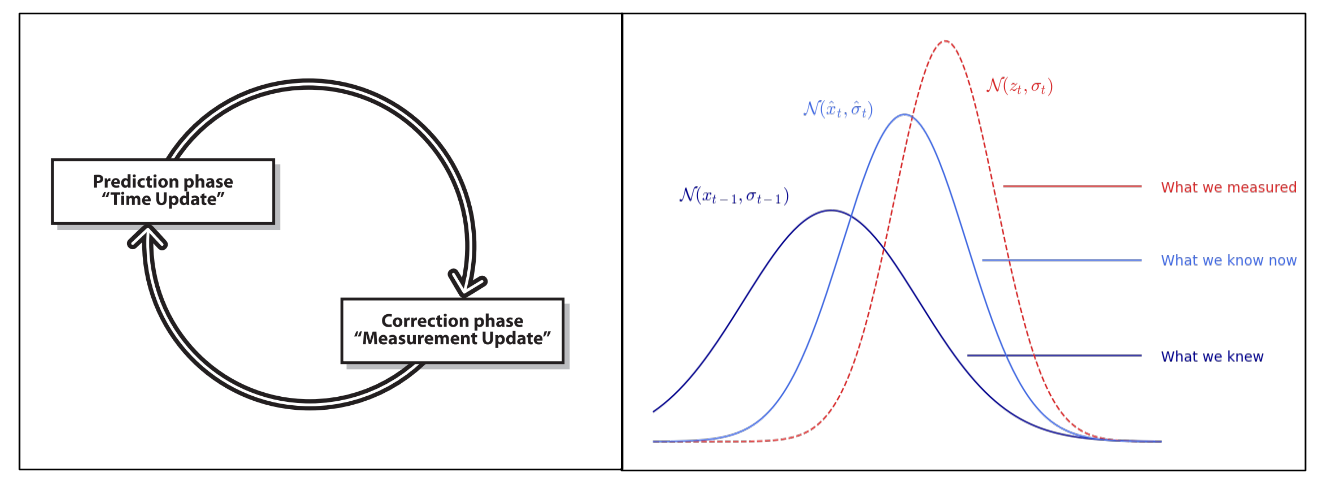
We previously considered the case of a static system in a state $x$ as well as a series of measurements of this system. In a dynamic case where the state of the system varies over time, we divide the estimation of the Kalman filter into 2 steps:
- the prediction phase: we use past information and the dynamic model to predict the next state of the system. We also predict the error covariance. It models the state of the system.
- the correction phase or update: we combine the prediction made with a new measurement to refine the model and the estimate of the state of the system as well as the covariance of the error. It models the measurement of the system.
For example, if we measure the position of a car at time $t-1$ then at time $t$. If the car has a speed $v$ then we do not directly integrate the new measurement directly. First, we fast-forward our model based on what we knew at time $t-1$ to have a prediction of the state at time $t$. In this way, the new measurement acquired at time $t$ is merged not with the old model of the system but with the old model of the system projected forward at time $t$
Starting from the hypothesis that the dynamics of the modeled system is linear, the prediction phase is then written:
\[\left. \begin{aligned} \hat x_t &= a \ \hat x_{t-1} \\ \hat \sigma_t^2 &= a^2 \ \hat \sigma_{t-1}^2 \\ &\scriptsize \color{blue} \text{due to $var(ax+b) = a^2 var(x)$} \end{aligned} \right.\]And the correction phase calculated in the previous section:
\[\left. \begin{aligned} \hat x_t &= \hat x_{t-1} + K (z_t - \hat x_{t-1}) \\ \hat \sigma_t^2 &= (1 - K) \hat \sigma_{t-1}^2 \\ \end{aligned} \right.\]
Generalization
We can extend the previous equations to the multidimensional case where the state of our system is defined by several quantities. We then seek to estimate the state of the system $\hat X \in \mathbb{R}^d$ at instant $t$ and its covariance matrix associated $\hat P \in \mathbb{R}^{d \times d}$ (with $d$ the dimension of the system). The equations become:
prediction phase
\[\left. \begin{aligned} \hat X_t &= A \hat X_{t-1} \\ \hat P_t &= A P_{t-1} A^T + Q \end{aligned} \right.\]where $A \in \mathbb{R}^{d \times d}$ is the state transition matrix modeling the dynamics of the system and $Q \in \mathbb{R}^{d \times d}$ the process noise covariance matrix capturing errors not modeled by $A$ (the larger it is, the more we trust the measurements rather than the predictions of the dynamic model).
correction phase
\[\left. \begin{aligned} \hat X_t &= \hat X_t + K(Z_t - \hat X_t) \\ \hat P_t &= \hat P_t - K \hat P_t \end{aligned} \right.\]with the Kalman gain $ K = \hat P_t (\hat P_t + R)^{-1} $
where $Z \in \mathbb{R}^d$ is the measurement of the system (or observation) and $R \in \mathbb{R}^{d \times d}$ the covariance matrix of the measurement which models l measurement error.
There are more sophisticated versions of the Kalman filter that can take as input a $U$ command sent to the system. We also frequently find the observation matrix $H \in \mathbb{R}^{d \times m}$ linking the real state of the system to the observed variables, in fact we can model a system with $d$ dimensions but only observe $m$ of its variables ($m<d$). The prediction phase remains the same but the correction phase is then:
\[\begin{aligned} \hat X_t &= \hat X_t + K(\textcolor{blue}{H} Z_t - \hat X_t) \\ \hat P_t &= \hat P_t - K \textcolor{blue}{H} \hat P_t \end{aligned}\]with the Kalman gain $ K = \hat P_t \textcolor{blue}{H^t} (\textcolor{blue}{H} \hat P_t \textcolor{blue}{H^T} + R)^{-1 } $
Examples
The Kalman filter is a generic tool and these equations can easily be implemented in a few lines:
def kalman_estimation(X_est, P_est, Z_obs):
     # state prediction
     X_est = A @ X_est
     P_est = A @ P_est @ A.T + Q
     # observation
     Z_pred = H @ X_est
     #kalmangain
     K = P_est @ H.T @ np.linalg.inv(H @ P_est @ H.T + R)
     # phase correction
     if Z_obs:
       X_est = X_est + K @ (Z_obs - Z_pred)
       P_est = P_est - K @ H @ P_est
     # final return estimate
     return X_est, P_est
Note: If the observation is not available at time $t$, we only execute the prediction phase of the Kalman filter to have an estimate using the dynamic model.
However, the crucial part of the problem most of the time lies in setting the system parameters $A$, $Q$, $H$ and $R$ so that the filter works correctly. In addition, it can become powerful when it allows you to estimate a quantity that is not measured, as in the examples below with the speed of an object and the bias of a gyroscope.
Object tracking (Tracking)
We want to implement a Kalman filter applied to an object tracking problem on an image. The object is spotted by a basic object detector by looking at a color interval in HSV space which returns the position $(x,y) \in \mathbb{N}^2$ in pixels in the image.
def simple_detector(image):
     # go to HSV space
     image = cv2.cvtColor(image, cv2.COLOR_BGR2HSV)
     # look into interval
     mask = cv2.inRange(image, np.array([155, 50, 50]) , np.array([170, 255, 255]))
     # sort by contour
     obj = cv2.findContours(mask, cv2.RETR_EXTERNAL, cv2.CHAIN_APPROX_SIMPLE)[-2]
     obj = sorted(obj, key=lambda x:cv2.contourArea(x), reverse=True)
     # keep center point
     if obj:
         (cX, cY), _ = cv2.minEnclosingCircle(obj[0])
         Z = [cX, cY]
     # return empty if no detection
     else:
         Z = []
     return Z
At each instant $t$, the movements of the object are modeled by the following equation of motion:
\[x_{t+1} = x_t + \Delta t \ \dot x_t\]where $\Delta t \in \mathbb{R}$ is the time step, $x_t$ the position and $\dot x_t$ the speed of the object at $t$. The state of the system is described by the position and the velocity in 2 dimensions: $ X_t = \begin{bmatrix} x_t & y_t & \dot x_t & \dot y_t \end{bmatrix}^T $. To obtain the state transition matrix $A$, we write the dynamics of the system in matrix form:
\[\begin{array}{cc} &\Rightarrow& \left\{ \begin{array}{cc} x_{t+1} &=& x_t &+& 0 y_t &+& \Delta t \ \dot x_t &+& 0 \dot y_t \\ y_{t+1} &=& 0 x_t &+& y_t &+& 0 \dot x_t &+& \Delta t \ \dot y_t \\ \dot x_{t+1} &=& 0 x_t &+& 0 y_t &+& \dot x_t &+& 0 \dot y_t \\ \dot y_{t+1} &=& 0 x_t &+& 0 y_t &+& 0 \dot x_t &+& 1 \dot y_t \end{array} \right. \\ \\ \\ &\Rightarrow& \begin{array}{cc} X_{t+1} &=& \underbrace{ \begin{bmatrix} 1 & 0 & \Delta t & 0 \\ 0 & 1 & 0 & \Delta t \\ 0 & 0 & 1 & 0 \\ 0 & 0 & 0 & 1 \\ \end{bmatrix}}_A X_t \end{array} \end{array}\]Furthermore, the detector allows only the position $(x,y)$ to be obtained but not the speed $(\dot x, \dot y)$, the observation matrix is therefore $H = \begin{bmatrix} 1 & 0 & 0 & 0 \\ 0 & 1 & 0 & 0 \end{bmatrix} $ to relate only the first 2 variables of the system to our observation. The parameters $Q$ and $R$ can also be refined depending on the noise of our detector and the model. In python, we have:
# Initial state
X = np.array([500, 500, 0, 0]) # can be adjusted with 1st observation
P = np.eye(4)

# Kalman parameters
dt = 0.1
A = np.array([[1, 0, dt, 0], [0, 1, 0, dt], [0, 0, 1, 0], [0, 0, 0, 1]])
H = np.array([[1, 0, 0, 0], [0, 1, 0, 0]])
Q = np.eye(4)
R = np.eye(2)
We open the video and for each frame, we detect the position of the object then we apply the Kalman filter. It allows us to have access to the speed of the system which is not observed. Speed is represented in the example below by the arrow. Furthermore, if the detection fails and the position of the object is not available at time $t$, we only execute the prediction phase of the Kalman filter to still have an estimate using the dynamic model.
# open video
cap = cv2.VideoCapture(r'path\to\my\video.mp4')
#loop on video frame
while True:
     #getframe
     ret, frame = cap.read()
     if not ret:
         break
     # simple object detection
     Z_obs = simple_detector(frame)
     # kalman filter
     X, P = kalman_estimation(X, P, Z_obs)
     #displaying
     plt.imshow(cv2.cvtColor(frame, cv2.COLOR_BGR2RGB))
     plt.plot(Z_obs[0], Z_obs[1], 'r.', label="detected")
     plt.plot(X[0], X[1], 'g.', label="kalman")
     plt.arrow(X[0], X[1], X[2], X[3], color='g', head_length=1.5)
     plt.legend(loc="upper right")
     plt.axis("off")
# close video
cap.release()
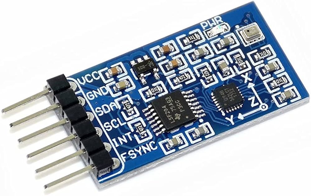
Inertial unit (IMU)
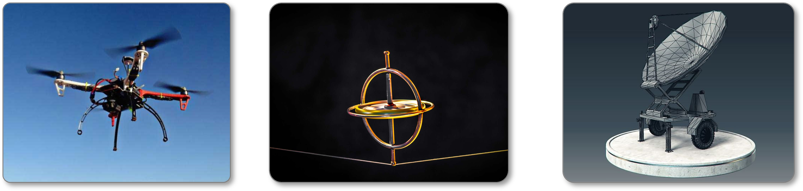
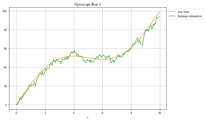
The Inertial Measurement Unit are electronic sensors that are found almost everywhere these days (phones, drones, planes, Nintendo Wii, etc.), they allow us to measure the acceleration and angular speed of an object to then estimate the orientation and position by integration. Acceleration is measured by an accelerometer and angular velocity by a gyroscope, but the difficulty comes from the fact that the gyroscope has a bias that changes over time. If we do not correct this drift, we will have the impression that the object is tilting slowly when in reality, it is not moving!
The dynamics of the system is modeled as in the previous example with the equation of angular motion:
\[\alpha_{t+1} = \alpha_t + \Delta t \ \dot \alpha_t\]where $\Delta t \in \mathbb{R}$ is the time step, $\alpha_t$ the angle and $\dot \alpha_t$ the angular velocity. The state of the system is, ultimately, described by the angle, the angular velocity and the bias $b$ (which we do not observe): $X_t = \begin{bmatrix} \alpha_t & \dot \alpha_t & b_t \end{bmatrix}^T$. Not knowing the model of evolution of the bias $b$ of the gyroscope, we consider it fixed here. We then have in matrix form:
\[X_{t+1} = \underbrace{\begin{bmatrix} 1 & \Delta t & 0 \\ 0 & 1 & 0 \\ 0 & 0 & 1 \end{bmatrix}}_A X_t\]Note: Here we model a simplistic case where the accelerometer gives us directly $\alpha$, the angle of inclination in relation to the gravitational force (which is nothing other than an acceleration !), the object rotates but does not move. By orienting it towards the ground (along the Z axis), we obtain an acceleration of 9.8 m/s², the constant $g$. To obtain a measure of the orientation angle, it is therefore sufficient to take $-\arcsin(a_{measure}/g)$.
As stated previously, the bias $b$ is not a quantity observed by our IMU. The observation matrix appears clearly by writing the relation linking the biased observation of the angular velocity $\dot \alpha_{observed} = \dot \alpha_{true} + b$. That’s to say :
\[\underbrace{\begin{bmatrix} \alpha \\ \dot \alpha + b \end{bmatrix}}_{observation} = \underbrace{\begin{bmatrix} 1 & 0 & 0 \\ 0 & 1 & 1 \end{bmatrix}}_H \quad \underbrace{\begin{bmatrix} \alpha \\ \dot{\alpha} \\ b \end{bmatrix}}_X\]Finally, we must determine how to fill $R$, the measurement noise and $Q$, the model noise. The matrix $R$ is simply composed of the noise of the sensors on the diagonal (no covariance because sensors are uncorrelated with each other) i.e. $R = \begin{bmatrix} \sigma_1^2 & 0 \\ 0 & \sigma_2^2 \end{bmatrix}$. The matrix $Q$ represents the modeling errors of $A$: for example we modeled that the bias $b$ and that the angular velocity $\dot \alpha$ were constant, which is false, we will put terms fairly raised at these locations and we will refine them empirically based on the problem data. On the other hand, the error of the model on the angle $\alpha$ can be set to $0$ since the state equation perfectly determines its value as a function of $\dot \alpha$. Here, we have $Q = \begin{bmatrix} 0 & 0 & 0 \\ 0 & \epsilon_{\dot \alpha} & 0 \\ 0 & 0 & \epsilon_b\end{bmatrix} = \scriptsize \textcolor{blue}{\begin{bmatrix}0 & 0 & 0 \\ 0 & 3 & 0 \\ 0 & 0 & 5 \end{bmatrix} \leftarrow \textit{empirically determined}}$
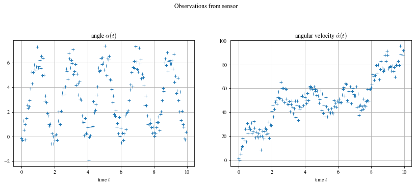
In Python, I start by synthetically generating the problem data. The angle is a sinusoidal function with a bias which evolves over time and the angular speed is its derivative, we add Gaussian noise to this data to have our observation vector, the measurement which comes out of the sensors.
dt = 0.05 # time step
T = 10 # total time
N = int(T/dt) # number of data
times = np.arange(0, T, dt) # time array
# Define state vector to be estimated (normally unknown)
X_true = np.zeros((N, 3))
X_true[:, 0] = -1 * np.pi * np.cos(np.pi * times) + np.pi
X_true[:, 1] = np.diff(X_true[:,0], prepend=-np.pi*dt)/dt # velocity as derivative of position
X_true[:, 2] = 10 * times + 20 * np.sin(2 * np.pi * 0.1 * times)
# Noise sensors
noise = np.zeros((N,2))
s = np.array([np.pi**2 * 0.06, np.pi * 0.2])
noise[:,0] = s[0] * np.random.randn(N)
noise[:,1] = s[1] * np.random.randn(N)
# Generate observation
X_obs = np.zeros((N, 2))
X_obs[:, 0] = X_true[:, 0] + noise[:,0]
X_obs[:, 1] = X_true[:, 1] + X_true[:, 2] + noise[:,1]
We can then declare the Kalman parameters defined previously and initialize the state variable and its covariance estimated by the filter (here, X_est and P_est). Additionally, I save the history of values in X_kalman.
#Kalman filter parameter
H = np.array([[1,0,0],[0,1,1]])
R = np.array([[s[0]**2,0],[0,s[1]**2]])
A = np.array([[1,dt,0],[0,1,0],[0,0,1]])
Q = np.array([[0,0,0],[0,3,0],[0,0,5]])
# initial state
X_est = np.zeros(3)
P_est = np.zeros((3,3))
X_kalman = np.zeros((N, 3))
# loop over time
for t in range(2,N):
     X_est, P_est = kalman_estimation(X_est, P_est, X_obs[t, :].T)
     # save history
     X_kalman[t, :] = X_est
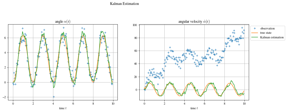
Having synthetically generated the data, the real state of the system is available (which is not the case in practice). We can therefore compare the error of the filter to the error if we took the measurement directly, we calculate the residuals $RSS = \sum_i^N (y_i - \hat y_i)^2$ and we have, for the Kalman filter , $RSS_{kalman} = [38; 2007]$ and, without filter, $RSS_{observation} = [80; 575873]$. The difference is obvious for the 2nd variable $\dot \alpha$ where the bias is taken into account by Kalman.
For further
An important limitation of the filter presented here is that it models a linear dependence with time, which is quite rare in practice. We can still use it and obtain good results as shown in the examples above but there is a non-linear version called extended Kalman filter where $A$ is replaced by a non-linear and differentiable function $f$ in the state prediction equation and its Jacobian $F=\frac{\partial f}{\partial x}$ in the equation of covariance prediction. This solution is generally used in navigation systems and GPS but we note that it can sometimes be unstable (divergence) depending on the initialization of the initial state unlike the linear version.
Another advantage of the Kalman filter is being able to do sensor fusion. A very simple example would be to have a system where we have access to 2 noisy sensors measuring the same size, for example a radar and a GPS which measure the position $x$ we would have the observation matrix $H$ via $\begin{bmatrix} x_{radar} \\ x_{GPS} \end{bmatrix} = \underbrace{\begin{bmatrix} 1 & 0 \\ 1 & 0 \end{bmatrix}}_H \begin{bmatrix} x \\ \dot x \end{bmatrix}$, and we would thus benefit from the 2 information from the 2 different sensors in our predictions.
![]()
![]()
![]()
![]()
Laisser un commentaire