CNN: convolution, Pytorch, Deep Dream

9 minute(s) de lecture

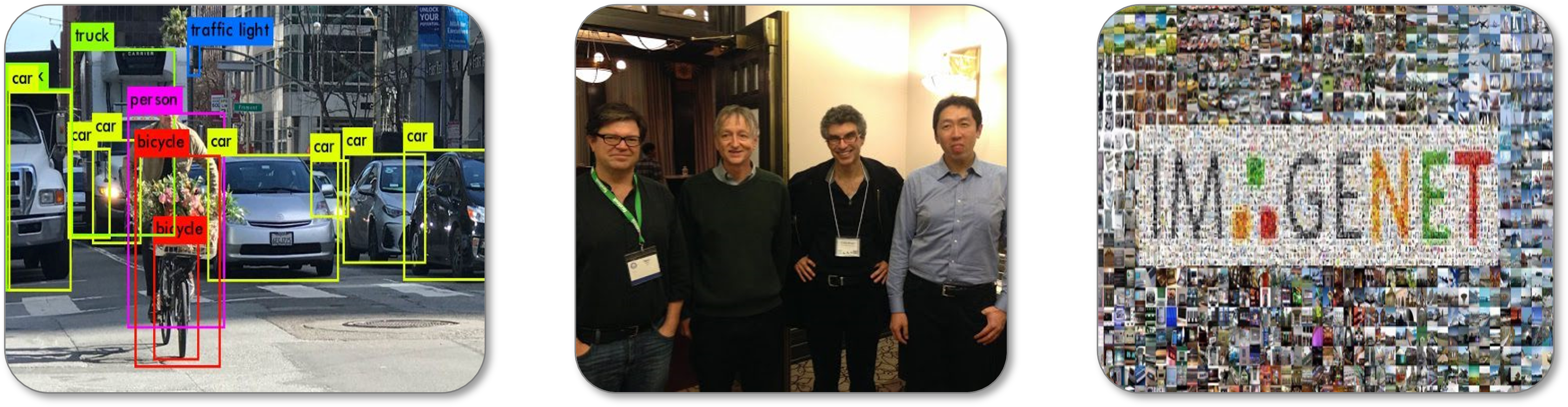
Convolutional neural networks (CNN) are the models that have made it possible to make a leap forward in image recognition problems. They are at the heart of many applications ranging from facial identification security systems to the classification of your vacation photos, including synthetic face generation and Snapchat filters. One of the founders of this model is Yann Le Cun (a Frenchman!) who, in 1989, applied gradient backpropagation to learn convolution filters and enabled a neural network to recognize handwritten digits. However, it was only in 2012 that CNNs spread widely in the computer vision scientific community with Alex Krizhevsky designing the AlexNet architecture and winning the ImageNet Large Scale Visual Recognition Challenge competition (1 million images of 1000 different classes) by implementing its algorithm on GPUs which allows the model to learn quickly from a large quantity of images. This model achieves 10% higher performance than all the others at this time and it is now one of the most influential published papers in Computer Vision (in 2021, more than 80,000 citations according to Google Scholar).

Convolutions and Neural Networks

Completely connected neural network models (see previous post) are not suitable for solving image processing problems . Indeed, MLPs have each neuron of a layer connected to each input unit: the number of parameters to learn quickly becomes high and a strong redundancy in the weights of the network can exist. Moreover, to use an image in such a network, all the pixels would have to be transformed into a vector and no information on the local structure of the pixels would then be taken into account.

The convolution product, denoted $\ast$, is an operator which generalizes the idea of a moving average. It applies both to temporal data (in signal processing for example) and to spatial data (in image processing). For the case of images, i.e. discrete and in 2 dimensions, the convolution between an image $I$ and a kernel $w$ (or kernel) can be calculated as follows:

\[I(i,j) * \omega =\sum_{x=-a}^a{\sum_{y=-b}^b{ I(i+x,j+y)} \ \omega(x ,y)}\]

The idea is to drag the kernel spatially over the entire image and each time to make a weighted average of the pixels of the image found in the window concerned by the elements of the kernel. Depending on the value of the elements of the convolution kernel $w$, the operation can highlight particular characteristics found in the image such as contours, textures, shapes.

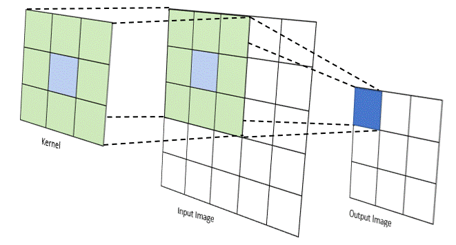
Note: There are several parameters associated with the convolution operation like the size of the kernel used, the step size when dragging the window over the image, the way we handle the edges of the image, the rate of core expansion… more info here

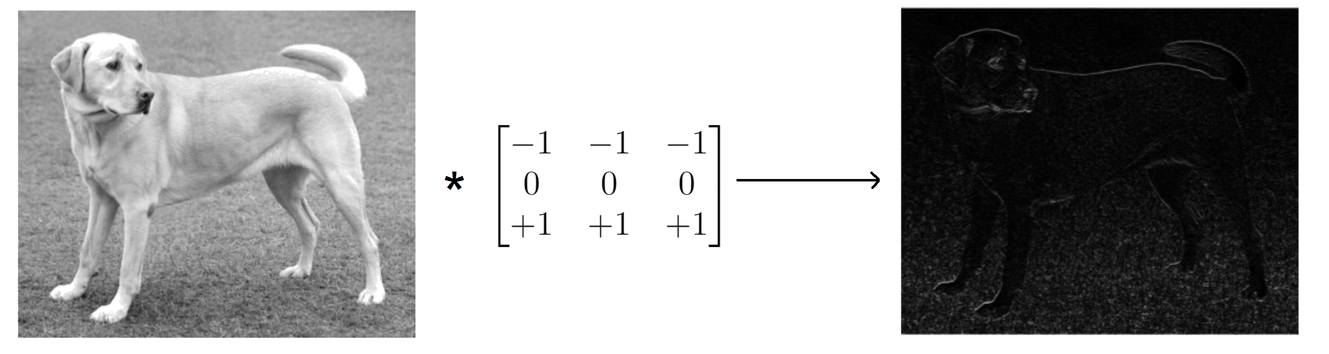
For example, we can highlight the pixels of an image corresponding to the horizontal contours by applying a convolution with a kernel of size $3 \times 3$ with $-1$ in the 1st line, $0$ in the 2nd line and $+1$ in the 3rd row of the matrix.

import matplotlib.pyplot as plt
import numpy as np
from scipy.signal import convolve2d
#readimage
image = np.array(Image.open("path/to/file.jpg").convert('L'))
# apply convolution
kernel = np.array([[-1, -1, -1],
                   [0, 0, 0],
                   [+1, +1, +1]])
conv_output = convolve2d(image, kernel, mode='same')
# display
plt.figure(figsize=(15.5))
plt.subplot(121), plt.imshow(image, cmap='gray'), plt.axis('off')
plt.subplot(122), plt.imshow(np.abs(conv_output), cmap='gray'), plt.axis('off')
plt.tight_layout()
plt.show()

The idea of the CNN model architecture is to keep completely connected layers for classification. However, at the inputs of these layers, the image is not directly used, but the output of several convolution operations which aim to highlight the different characteristics of an image by encoding the objects in a certain way. which are present or not. In particular, multi-channel convolutions are used which consist in applying a standard convolution to each channel of the input then summing each convolution product obtained to obtain a single 2D matrix. For example for a color image the channels are red, green and blue, we then have 3 kernels to convolve with the associated channels then the 3 products obtained are summed.

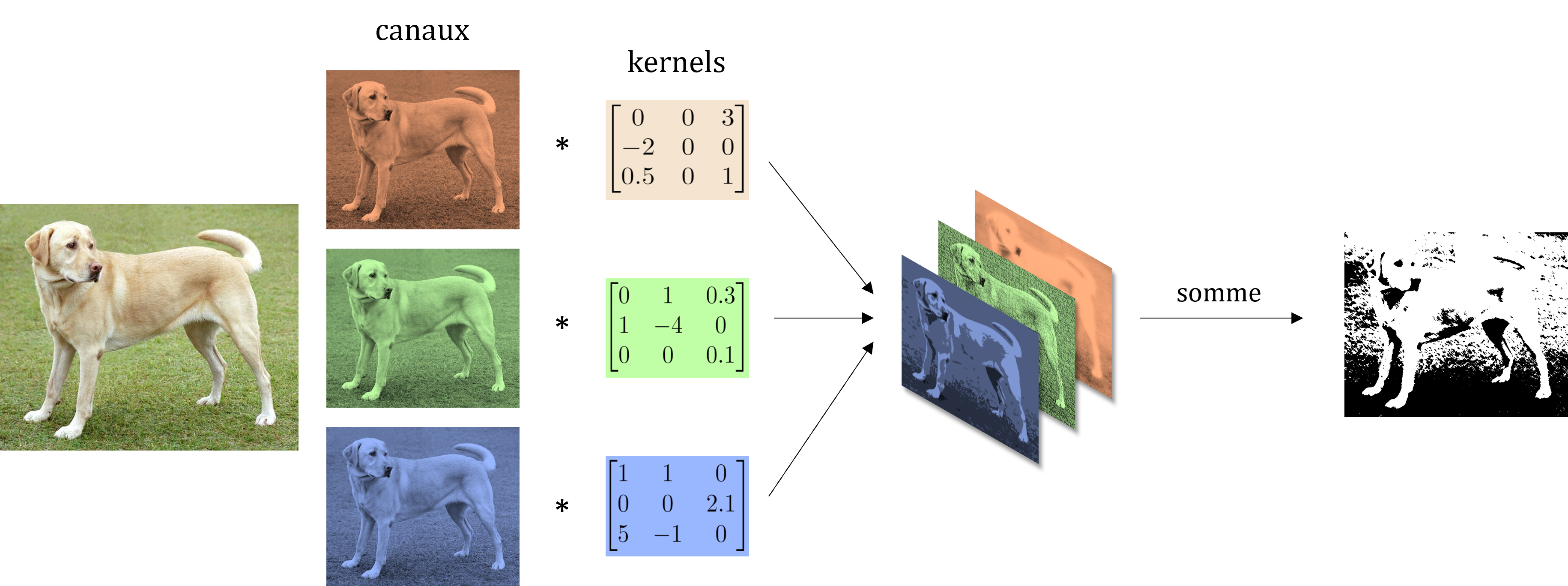
Note: In 2D (1 channel only), we use the term kernel to talk about the kernel. In 3D (more than one channel), we use the term filter which is made up of as many kernels as the number of channels of the input volume.

More precisely in CNNs, a convolutional layer is composed of a set of $N_f$ filters of size $N_W$ x $N_H$ x $N_C$ plus a bias per filter followed by a nonlinear activation function. Here, $N_W$ and $N_H$ designate the spatial sizes of the filter while $N_C$ is the number of channels (sometimes called feature map). Each filter performs a multi-channel convolution, we then obtain $N_f$ convolution products which are concatenated in an output volume. These $N_f$ products then become the channels of the next volume which will pass into the next convolutional layer. Note that the depth of the filters must necessarily correspond to the number of channels of the input volume of each layer but the number of filters is an architecture hyperparameter of the model. In the end, the sequence of these multichannel convolutions creates at output a volume of features (features) of the input image, these features are then passed to the fully connected network for classification.

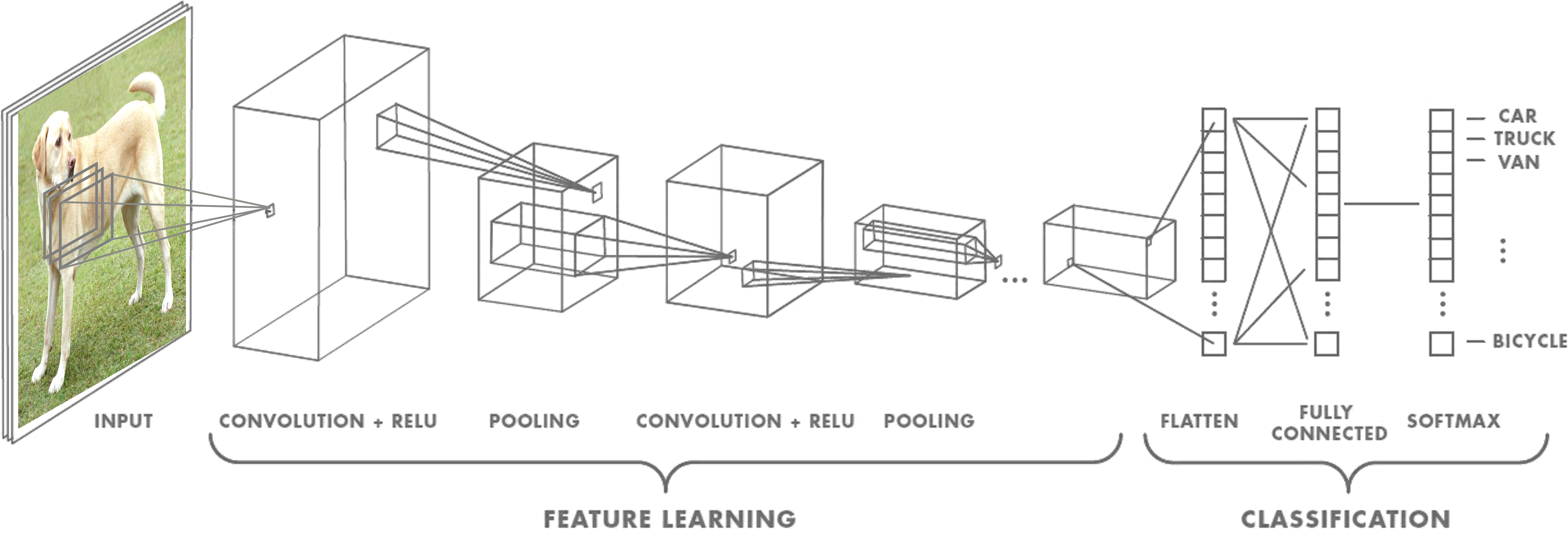
Important: A convolutional layer is usually composed (in addition to convolution) of a nonlinear activation function and sometimes other types of operations (pooling, batch-normalization, dropout…).

In the previous post, we defined an MLP and its training from zero. Here, the PyTorch library is used. It allows to easily build neural networks by taking advantage of its automatic differentiation engine for the training as well as its many specialized functions (like the convolution).

import torch
import torch.nn as nn
import torch.nn.functional as F
from torch import optim

class My_Custom_Model(nn.Module):

    def __init__(self):
        ''' define some layers '''
        super().__init__()
        # feature learning
        self.conv1 = nn.Conv2d(3, 6, 5)
        self.pool = nn.MaxPool2d(2, 2)
        self.conv2 = nn.Conv2d(6, 16, 5)
        # classification
        self.fc1 = nn.Linear(16*5*5, 120)
        self.fc2 = nn.Linear(120, 84)
        self.fc3 = nn.Linear(84, 10)

    def forward(self, x):
        ''' create model architecture - how operations are linked '''
        x = self.pool(F.relu(self.conv1(x)))
        x = self.pool(F.relu(self.conv2(x)))
        x = torch.flatten(x, 1)
        x = F.read(self.fc1(x))
        x = F.read(self.fc2(x))
        x = self.fc3(x)
        return x

As you may have understood, what is interesting with these convolution operations is that the weight of the filters can be learned during the optimization by backward propagation of the gradient since it is possible to calculate in an exact way the value of $ \frac{\ partial\mathcal{L}}{\partial W}$ by chain derivation.

# define loss and optimizer
criterion = nn.CrossEntropyLoss()
optimizer = optim.SGD(my_cnn_model.parameters(), lr=0.001)
# training loop
num_epochs = 100
for epoch in range(num_epochs):
    for i, data in enumerate(train_loader):
        images, labels = data
        # Forward pass
        output = model(images)
        loss = criterion(outputs, labels)
        # Backward pass
        optimizer.zero_grad()
        loss.backward()
        # optimization step
        optimizer.step()

Note: For large input data, we often use as an optimization algorithm a stochastic gradient descent where the loss is approximated by using a batch of some data (for example, 8, 16 or 32 pictures).

Deep Dream

One of the challenges of neural networks is to understand what exactly is happening at each layer. Indeed, their cascade architecture as well as their numerous interconnections make it not easy to interpret the role of each filter. The visualization of features is a line of research that has developed in recent years, which consists of finding methods to understand how CNNs see an image.

DeepDream is the name of one of these techniques created in 2015 by a team of engineers from Google, the idea is to use a network already trained to recognize shapes to modify an image so that a given neuron returns an output higher than the others. The algorithm looks like classic backpropagation but instead of modifying the weights of the network we adjust the pixels of the input image. Moreover, the optimization criterion is not a cross entropy but directly the norm of the output of the neuron to be visualized (it can be the entire layer or a filter) that we will seek to maximize, we then make a rise gradient (we could also minimize the opposite).

# Parameters
iterations = 25 # number of gradient ascent steps per octave
at_layer = 26 # layer at which we modify image to maximize outputs
lr = 0.02 # learning rate
octave_scale = 2 # image scale between octaves
num_octaves = 4 # number of octaves

# Load Model pretrained
network = models.vgg19(pretrained=True)
# Use only needed layers
layers = list(network.features.children())
model = nn.Sequential(*layers[: (at_layer + 1)])
# Use GPU is available
device = torch.device("cuda:0" if torch.cuda.is_available() else "cpu")
model = model.to(device)

An additional trick to obtain an interesting visualization is to operate at different spatial resolutions, here we speak of octave. In addition, the loss is normalized at all layers so that the contribution of large layers does not outweigh that of small layers.

# loop on different resolution scale
detail = np.zeros_like(octaves[-1])
for k, octave_base in enumerate(tqdm(octaves[::-1], desc="Octaves : ")):
    # Upsample detail to new octave dimension
    if k > 0: 
      detail = nd.zoom(detail, np.array(octave_base.shape)/np.array(detail.shape), order=1) 
    # Add detail from previous octave to new base
    input_image = octave_base + detail
    # Updates the image to maximize outputs for n iterations
    input_image = Variable(torch.FloatTensor(input_image).to(device), requires_grad=True)
    for i in trange(iterations, desc="Iterations : ", leave=False):
        model.zero_grad()
        out  = model(input_image)
        loss = out.norm()
        loss.backward()
        # gradient ascent
        avg_grad = np.abs(input_image.grad.data.cpu().numpy()).mean()
        norm_lr  = lr/avg_grad
        input_image.data = input_image.data + norm_lr * input_image.grad.data
        input_image.data = clip(input_image.data)
        input_image.grad.data.zero_()
        # Extract deep dream details
        detail = input_image.cpu().data.numpy() - octave_base

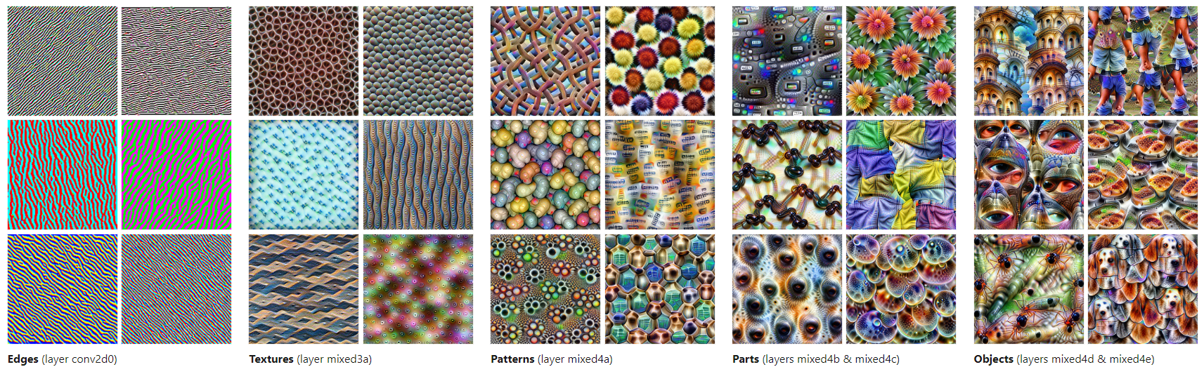
Depending on the number of iterations, we obtain more and more abstract images with psychedelic shapes that appear as and when the name DeepDream. In fact, these abstract shapes are present especially for the deeper layers, the first layers usually accentuate simple features like edges, corners, textures…

With this tool, one can create very advanced artistic effects like on DeepDreamGenerator’s instagram. But we can also accentuate the pscychedelic effect by doing a lot of iterations or by feeding the output of the algorithm as input several times. And with a little effort, one can manage to visualize what it is like to go to the supermarket in these dreams from very real images.

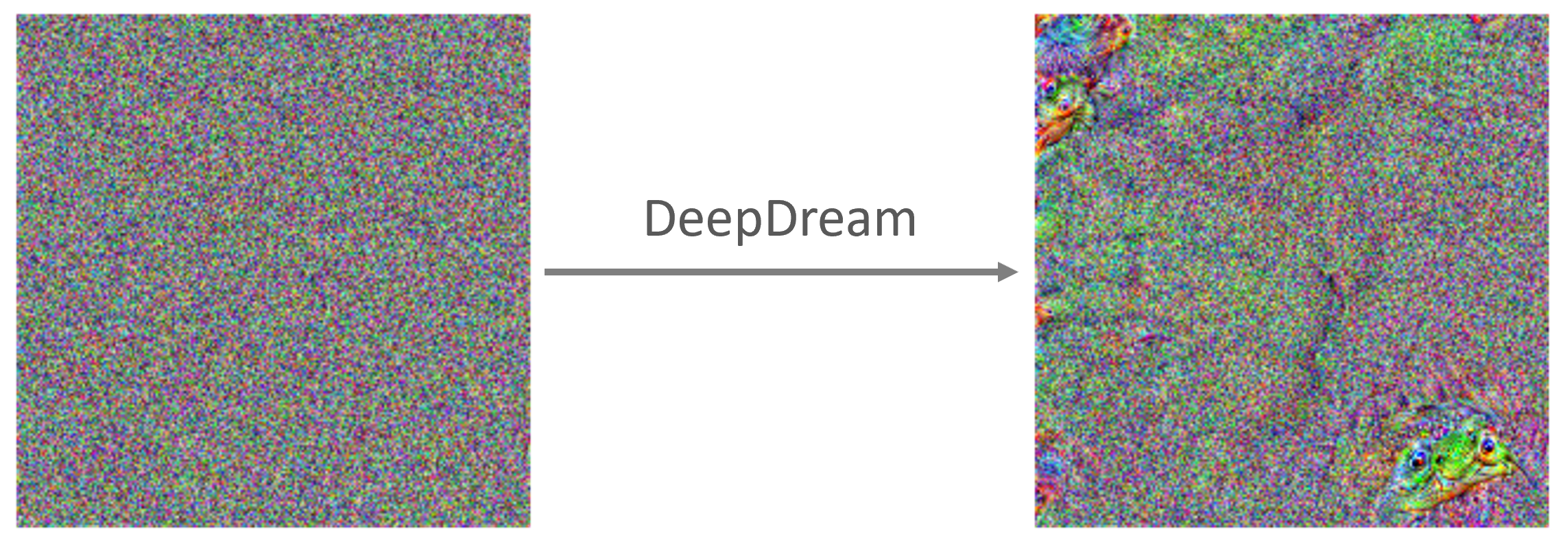
As presented above, Deep Dream has a drawback if you want to run it on an input white noise image to visualize what might emerge and thus have a more accurate representation of CNN features. Indeed, it can be seen that the image then remains dominated by high-frequency patterns.

Generally, to counter this effect, what works best is to introduce regularization in one way or another into the model. For example, transformation robustness tries to find examples that always strongly activate the optimization function when they are very weakly transformed. Concretely, this means that we shake, rotate, decrease or increase the image randomly before applying the optimization step. The lucid (tensorflow) and lucent (pytorch) libraries are open-source packages that implement all kinds of visualization methods.

# load libraries
from lucent.optvis import render
from lucent.modelzoo import vgg19
#loadmodel
model = vgg19(pretrained=True)
model = model.to(device)
model.eval()
# run optimization
image = render.render_vis(model, "features:30",thresholds=[100],show_inline=True)