

Neural Network: statistics, gradient, perceptron
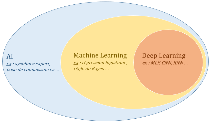
In recent years, we hear more and more in the media the words: artificial intelligence, neural network, Deep Learning … Indeed, many innovations have emerged thanks to these technologies but that this hides really behind this terminology? Ever since the first programmable computers were designed, people have been amazed to see these computers solving tasks impossible for any human being. However, these problems were actually easy to describe by a formal list of mathematical rules. The real challenge for computers is to perform tasks that humans perform easily and intuitively but have much more difficulty in formally describing, such as recognizing language or faces. Nowadays, we call artificial intelligence (AI) any technique allowing to solve a more or less complex problem by means of a machine. Machine Learning and Deep Learning are fields of study of AI based on statistical theories.
Statistical Learning
Statistical learning (or Machine Learning) focuses on the study of algorithms that allow computers to learn from data and improve their performance at solving tasks without having explicitly programmed each of them. between them. Consider a set $(x_i,y_i)$ of $n$ training data (with $x_i$ a data and $y_i$ its class). The goal of supervised learning is to determine an estimate $h$ of $f$ using the available data $(x_i,y_i)$. We then distinguish two types of predictions depending on the nature of $Y$: if $Y \subset \mathbb{R}$, we speak of a regression problem and if $Y = {1,…, I}$ we are talking about a classification problem. To estimate the law $f$, a classical approach is the minimization of the empirical risk. Given a loss function $L(\hat{y},y)$ (also called cost, loss, goal function) that measures how well the prediction $\hat{y}$ of a model $h$ is different from the true class $y$ then the empirical risk is:
\[R_{emp}(h) = \frac{1}{n} \sum_{i=1}^n L\left(h(x_i),y_i\right)\]The principle of empirical risk minimization says that the learning algorithm must choose a model $\hat{h}$ which minimizes this empirical risk: $ \hat{h} = \arg \min_{h \in \mathcal{ H}} R_{emp}(h) $. The learning algorithm therefore consists in solving an optimization problem. The function to be minimized is an approximation of an unknown probability, it is made by averaging the data available and the more data there is, the more accurate the approximation will be. About the loss $L(\hat{y},y)$ function, we can theoretically use the 0-1 loss function to penalize errors and do nothing otherwise:
\[L(\hat{y},y) = \left\{ \begin{array}{ll} 1 & \text{if } \hat{y} \neq y \\ 0 & \text{if } \hat{y} = y \end{array} \right.\]But, in practice, it is better to have a continuous and differentiable loss function for the optimization algorithm. For example, the mean squared error (MSE) which is often chosen for regression problems, for example for a linear case where we want to find the best straight line passing through points. However, the MSE has the disadvantage of being dominated by outliers which can cause the sum to tend towards a high value. A loss frequently used in classification and more suitable is the cross-entropy (CE):
\[MSE = (y - \hat{y})^2 \quad \quad \quad CE = - y \log(\hat{y})\]def compute_loss(y_true, y_pred, name):
if name == 'MSE':
loss = (y_true - y_pred)**2
elif name == 'CE':
loss = -(y_true * np.log(y_pred) + (1-y_true) * np.log(1-y_pred))
return loss.mean()
Note: To solve this minimization problem, the most efficient way is to use a gradient descent algorithm (see previous post) but requires knowing the exact derivative of the Loss function. Recent Deep Learning libraries (Pytorch, Tensorflow, Caffe …) implement these optimization algorithms as well as self-differentiation frameworks
Now that the notion of learning has been defined, the most important element is to build a $h$ model capable of classifying or regressing data. One of the most well-known models today is that of neural networks.
Neural Networks
Perceptron
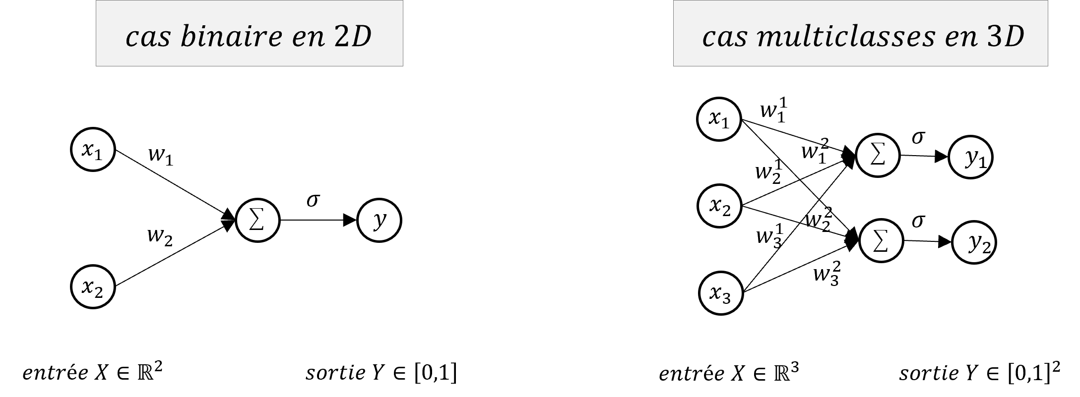
The first model at the origin of neural networks is the Perceptron (F. Rosenblatt, 1957), it can be seen as a single and simple neuron which solves a linear classification problem. The Perceptron transforms an input vector $X=(x_1,…,x_d) \in \mathbb{R}^d$ into an output $Y \in [0,1]$, the classification label. The idea is that we seek to separate our input space into 2 regions by a hyperplane $\mathcal{H}$ defined simply by:
\[\mathcal{H}: w^T X + b = 0 \iff \mathcal{H}: \sum_{i=1}^d w_i x_i + b = 0\]where $w=(w_1,…,w_d) \in \mathbb{R}^d$ and $b \in \mathbb{R}$ are the parameters of the hyperplane $\mathcal{H}$ that commonly called the weights of the neuron.
class Perceptron:
def __init__(self, n_inputs, n_iter=30, alpha=2e-4):
self.n_iter = n_iter # number of iterations during training
self.alpha = alpha # learning rate
self.w = np.zeros((n_iter, n_inputs+1))
self.w[0,:] = np.random.randn(n_inputs+1) # weights and bias parameters
def predict(self, X, i=-1):
return np.sign(X @ self.w[i,1:] + self.w[i,0])
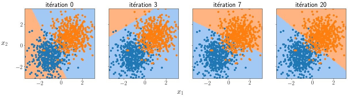
This hyperplane therefore separates the space into 2 and is therefore able to classify a datum $X$ by creating a rule like $ f(X) = 1 \ \text{si } w^T X + b<0 \ ; 0 \text{ otherwise} $. Our neuron model therefore boils down to parameters modeling a hyperplane and a classification rule. In our machine learning paradigm, we assume that we have, at our disposal, a set of $n$ data labeled $(X,Y) \in \mathbb{R}^{n\times d} \times [0 ,1]^n$. As explained in the previous section, the learning phase (or training phase) consists in minimizing the classification error made by the model on these data and adjusting the parameters $w$ and $b$ which allow the Perceptron model to correctly separate these data.
def gradient_descent(self, i, y, y_pred):
# construct input X and 1 to have bias
inputs = np.hstack((np.ones((X.shape[0], 1)), X))
# compute gradient of the MSE loss
gradient_loss = -2 * np.dot(y_true - y_pred, inputs)
# apply a step of gradient descent
self.w[i+1,:] = self.w[i,:] - self.alpha * gradient_loss
Above, the MSE loss was used. Its exact derivative as a function of $w$ can be calculated easily (see below).
$$ L = \frac{1}{n}\sum_{i=1}^n (y_i - \hat{y}_i)^2 = \frac{1}{n}\sum_{i=1}^n (y_i - (w_i x_i + b))^2 \\[5pt] \left\{ \begin{array}{ccc} \dfrac{\partial L}{\partial w} &=& \dfrac{\partial}{\partial w} \dfrac{1}{n} \sum_{i=1}^n (y_i - (w_i x_i + b))^2 \\[10pt] \dfrac{\partial L}{\partial b} &=& \dfrac{\partial}{\partial b} \dfrac{1}{n} \sum_{i=1}^n (y_i - (w_i x_i + b))^2 \\ \end{array} \right. \\[10pt] \left\{ \begin{array}{cc} \dfrac{\partial L}{\partial w} &=& -\dfrac{2}{m}\sum_{i=1}^{m}(y_i - w_i x_i - b)x_i \\[10pt] \dfrac{\partial L}{\partial b} &=& -\dfrac{2}{m}\sum_{i=1}^{m}(y_i - w_i x_i - b) \end{array} \right. \\[10pt] \left\{ \begin{array}{cc} \dfrac{\partial L}{\partial w} &=& -\dfrac{2}{m}\sum_{i=1}^{m}(y_i - \hat{y}_i)x_i \\[10pt] \dfrac{\partial L}{\partial b} &=& -\dfrac{2}{m}\sum_{i=1}^{m}(y_i - \hat{y}_i) \end{array} \right. \\ $$ In python, we added 1 to the input X to take into account the bias equation. The gradient is well written `gradient_loss = -2 * np.dot(y_true - y_pred, inputs)`Note that this model is very close to a simple linear regression but presented here for a classification problem, it can easily be adapted to a regression by removing the np.sign() function in the python code. On the other hand, the problem solved here is binary (we have 2 classes) but we can easily extend the model so that it predicts several classes by replacing the weight vector $w \in \mathbb{R}^d$ by a matrix $W \in \mathbb{R}^{d \times c}$ therefore representing several separating hyperplanes where $c$ is the number of possible classes, the output of the model $Y$ is no longer a scalar but then a vector of $\mathbb{R}^c$. Finally, note that in practice, the classification function $f$ is replaced by a differentiable function $\sigma: \mathbb{R} \rightarrow [0,1]$. For a binary problem, the sigmoid function $\sigma(z)=\frac{1}{1+e^{-z}}$ is used then the class is chosen according to a threshold (ex: $\sigma(z) > $0.5). For a multi-class case, the classification function is a softmax function $\sigma(z_j)=\frac{e^{z_j}}{\sum_{k=1}^Ke^{z_k}}$ which returns a vector of pseudo-probability (sum to 1) and the retained class is chosen by keeping the position of the maximum value of the vector.
Multi-Layer Perceptron
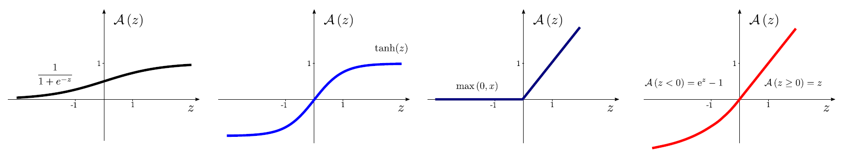
As described above, a single neuron can solve a linearly separable problem but fails when the data is not linearly separable. To approximate nonlinear behaviors, the idea is to add nonlinear functions in the model, they are called activation functions (see examples below).
def sigmoid(x):
return 1 / (1 + np.exp(-x))
def read(x):
return x * (x > 0)
def tanh(x):
return np.tanh(x)
The model of the neural network or Perceptron Multi-Layers consists in chaining successively several linear transformations carried out by simple neurons and nonlinear transformations carried out by these functions of activations until the last operation which will return the class predicted by the model. A layer $l$ of the neural network is then composed of $m$ neurons modeled by a weight matrix $W^l \in \mathbb{R}^{(d+1)\times m}$ (for simplicity we integrates the bias $b$ in $W$) as well as an activation function $A^l$. In the end, the complete neural network can be described by a combination of composition of functions and matrix multiplications going from the 1st layer to the last:
\[h(X) = \hat{Y} = A^l(W^l A^{l-1}(W^{l-1} \cdots A^0(W^0 X)\cdots))\]class MultiLayerPerceptron:
''' MLP model with 2 layers '''
def __init__(self, n_0, n_1, n_2):
# initialize weights of 1st layer (hidden) and 2nd layer (output)
self.W1 = np.random.randn(n_0, n_1)
self.b1 = np.zeros(shape=(1, n_1))
self.W2 = np.random.randn(n_1, n_2)
self.b2 = np.zeros(shape=(1, n_2))
def forward(self, X):
# input
self.A0 = X
# first layer
self.Z1 = np.dot(self.A0, self.W1) + self.b1
self.A1 = reread(self.Z1)
# second layer
self.Z2 = np.dot(self.A1, self.W2) + self.b2
self.A2 = sigmoid(self.Z2)
# output
y_pred = self.A2
return y_pred
Note: Note that we can build a network with as many hidden layers as we want and that each of these layers can also consist of an arbitrary number of neurons, regardless of the input dimension and out of the problem.
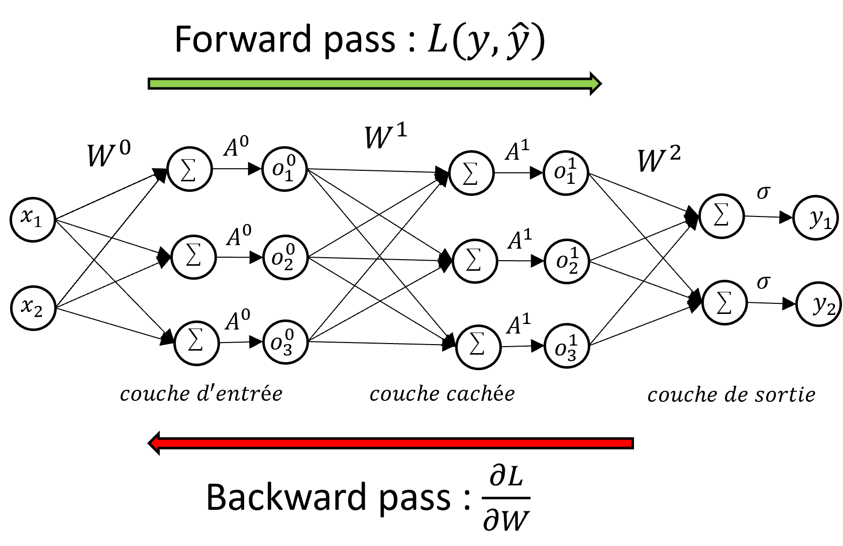
This sequence of layers of neurons poses a problem for the training phase: the calculation of $\frac{\partial\mathcal{L}}{\partial W}$ is less trivial than for the formal neuron model since it takes take into account the weights $W^l$ of each layer $l$. The gradient backpropagation technique allows to train multi-layered neural networks based on the chain derivation rule. The loss gradient is calculated using the derivatives of the weights of the neurons and their activation function starting from the last layer to the first layer. It is therefore necessary to browse the network forwards (forward pass) to obtain the value of the loss then backwards (backward pass) to obtain the value of the derivative of the loss needed by the optimization algorithm. If we are interested in the neuron $j$ of the layer $l$ towards the neuron $i$ of the layer $l+1$, we note $a$ the value of the vector product, $o$ the output of the neuron ( after activation) and keeping the rest of the previous notations, the calculation of the gradient of $L$ as a function of $W$ is:
\[\begin{align*} \dfrac{\partial L}{\partial w_{ij}^l} &= \underbrace{\quad \dfrac{\partial L}{\partial a_{j}^l} \ \ } \ \ \underbrace{\quad \dfrac{\partial a_j^l}{\partial w_{ij}^l} \quad} \\ & \qquad \ \ \ \delta_j^l \quad \ \ \ \dfrac{\partial}{\partial w_{ij}^l} \sum_{n=0}^{N_{l-1}} w_{nj}^l o_n^{l-1} = o_i^{l-1} \end{align*}\]We therefore have that the derivative $\dfrac{\partial L}{\partial w_{ij}^l}$ depends on the term $\delta_j^l$ of the layer $l$ and on the output $o_i^{l- 1}$ of layer $l-1$. This makes sense since the weight $w_{ij}^l$ connects the output of neuron $i$ in layer $l-1$ to the input of neuron $j$ in layer $l$. We now expand the term $\delta_j^l$:
\[\delta_j^l = \dfrac{\partial L}{\partial a_{j}^l} = \sum_{n=1}^{N_{l+1}} \dfrac{\partial L}{\partial a_n^{l+1}}\dfrac{\partial a_n^{l+1}}{\partial a_j^l} = \sum_{n=1}^{N_{l+1}} \delta_n^{l+1} \dfrac{\partial a_n^{l+1}}{\partial a_j^l}\]however, we have:
\[\begin{align*} & a_n^{l+1} &=& \sum_{n=1}^{N_{l}} w_{jn}^{l+1}A(a_j^l) \\ \Rightarrow & \dfrac{\partial a_n^{l+1}}{\partial a_j^l} &=& \ w_{jn}^{l+1}A'(a_j^l) \end{align*}\]and so:
\[\dfrac{\partial L}{\partial w_{ij}^l} = \delta_j^l o_i^{l-1} = A'(a_j^l) o_i^{l-1} \sum_{n=1}^{N_{l+1}} w_{jn}^{l+1} \delta_n^{l+1}\]We therefore obtain that the partial derivative of $L$ with respect to $w_{ij}$ at layer $l$ also depends on the derivative at layer $l+1$. To calculate the derivative of the entire network using the rule of chain derivation, it is therefore necessary to start with the last layer and end with the first, hence the term error backpropagation.
Warning: As the calculations of the backpropagation phase also depend on $a_j^l$ and $o_i^{l-1}$, you must first do a pass forward before the pass backward to store these values in memory.
''' training methods for 2 layer MLP and cross-entropy loss '''
def backward(self, X, y):
m = y.shape[0]
self.dZ2 = self.A2 - y
self.dW2 = 1/m * np.dot(self.A1.T, self.dZ2)
self.db2 = 1/m * np.sum(self.dZ2, axis=0, keepdims=True)
self.dA1 = np.dot(self.dZ2, self.W2.T)
self.dZ1 = np.multiply(self.dA1, d_relu(self.Z1))
self.dW1 = 1/m * np.dot(X.T, self.dZ1)
self.db1 = 1/m * np.sum(self.dZ1, axis=0, keepdims=True)
def gradient_descent(self, alpha):
self.W1 = self.W1 - alpha * self.dW1
self.b1 = self.b1 - alpha * self.db1
self.W2 = self.W2 - alpha * self.dW2
self.b2 = self.b2 - alpha * self.db2
Note: During training, only the weights $W$ of the model are optimized. The number of hidden layers as well as the number of neurons per layer are fixed and do not change. We are talking about hyperparameters, they must be chosen when designing the model. Optimal hyperparameter search techniques exist but are complex and computationally intensive.
Go further
The popularity of neural networks in recent years is actually not due to the MLP model presented so far. Indeed, the main drawback of MLP is the large number of connections existing between each neuron which leads to high redundancy and difficulty in training when the number of neurons and the input dimension are high.
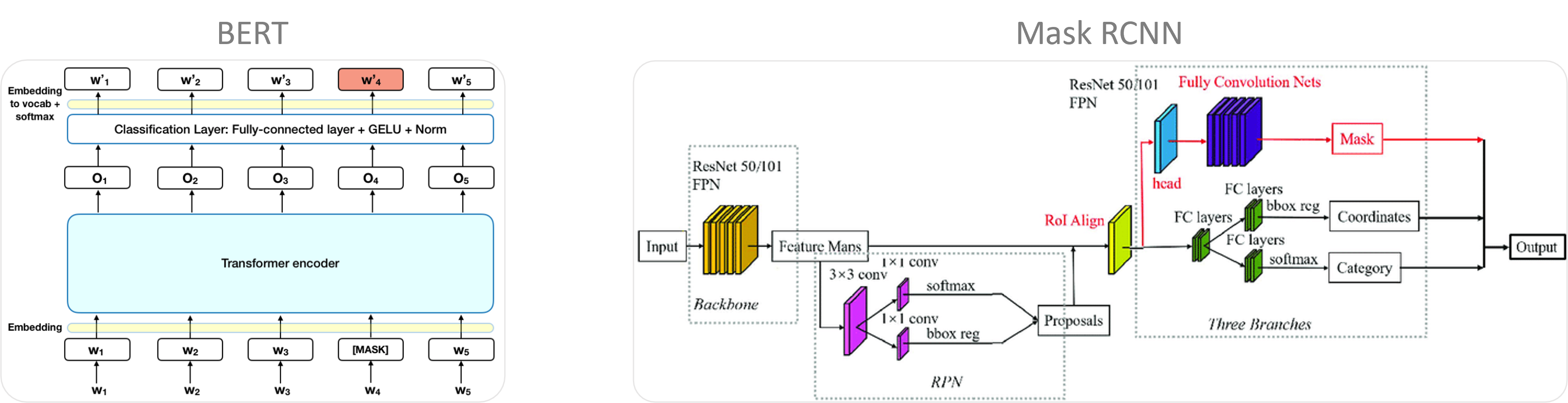
On complex problems such as image analysis, word processing or speech processing, the effectiveness of current neural networks is, for the most part, due to more advanced operations and connections that allow modeling and effectively represent these issues. For example, for images, convolution operators are exploited, they take advantage of the local pixel structure to understand the information present, ranging from simple shapes (lines, circles, color …) to more complex (animals, building , landscapes, etc.). For sequential data, LSTM (long short-term memory) connections are able to memorize important past data avoiding the problems of disappearance of gradient. On the other hand, many techniques exist to improve the learning phase and have performances that generalize the model to so-called test data never seen by the model during training (data augmentation, dropout, early stopping …).
![]()
![]()
![]()
![]()
Laisser un commentaire