

Optimization: algorithm, XFOIL, airfoil
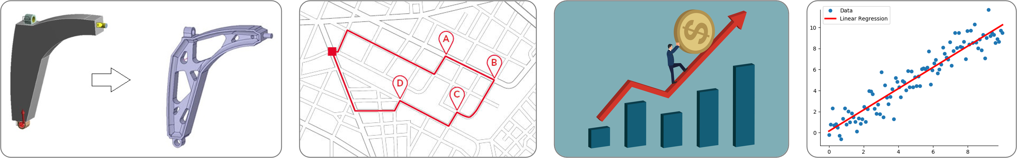
In everyday life, we often seek to optimize our actions to make the least effort and well, in the world of engineering, it’s the same thing. Minimization problems are ubiquitous in many systems whether to save time, money, energy, raw material, or even satisfaction. For example, we can seek to optimize a route, the shape of an object, a selling price, a chemical reaction, air traffic control, the performance of a device, the operation of an engine, etc. The complexity of the problems and their modeling makes optimization a very vast and varied branch of mathematics, in practice the quality of the results depends on the relevance of the model, the good choice of the variables that one seeks to optimize, the effectiveness of the algorithm and means for digital processing. In the field of aerodynamics, the shape of airplanes and racing cars is often designed so that the energy expended is minimal. After introducing some algorithmic aspects of the minimization problem, the following article will present how the profile of an aircraft wing can be optimized to maximize its performance.
Optimization algorithms
Faced with the resolution of an optimization problem, a 1st step is to identify to which category it belongs. Indeed, the algorithms are more or less adapted for given categories since the problem can be continuous or discrete, with or without constraints, differentiable or not, convex or not… We write an optimization problem without constraints simply:
\[\min_{x \in X} f(x)\]where $f$ can be called an objective function or a cost function. In theory, for unconstrained problems, one can find the minimum(s) by looking at when $ \nabla f(x) = 0 $ (first-order condition) and the positivity of the Hessian $H(x)$ (second order condition). For a problem with constraints, the Kuhn-Tucker conditions applied to the Lagrangian make it possible to transform the problem into a new one without constraints but with additional unknowns.
Note: A maximization problem can easily be transposed into a minimization problem: \(\max_{x \in X} f(x) \Leftrightarrow \min_{x \in X} - f(x)\)
For simple cases, we can solve the problem analytically. For example, when $f$ has a quadratic, linear and unconstrained form, canceling the gradient amounts to solving a linear system. But, in practice, the gradient may have a too complicated form or even the function $f$ may not have a known analytical form (it may be the result of a numerically solved PDE for example). There is therefore a wide variety of iterative optimization algorithms to try to find the minimum, some being more or less adapted to certain types of problem. On the other hand, it is common to validate these algorithms by testing them on known functions for which we know analytically the value of the true minimum, they make it possible to evaluate the characteristics of the approaches such as the speed of convergence, the robustness, the precision or general behavior. A fairly complete list of these test functions is available on wikipedia.
For the sake of simplicity, the 3 approaches below are simple approaches that introduce the basic notions of optimization algorithms, they will be tested on the Himmelblau test function. In reality, we most often call on libraries or specialized software that implement much more sophisticated approaches.
Gradient descent
 The gradient descent algorithm is used to minimize real differentiable functions. This iterative approach successively improves the sought point by moving in the direction opposite to the gradient so as to decrease the objective function. In its simple version, the algorithm finds a local minimum (and not a global one) and may have certain disadvantages such as the difficulty in converging if the parameter $\alpha$ (the step of the descent) is incorrectly set. There is a whole family of methods known as with descent directions which exploit the gradient to converge the minimum of $f$ more efficiently.
def gradient_descent(f, x0, gradient, alpha=0.01, itermax=1000):
# initialization
x, fx = np.zeros((itermax+1, len(x0))), np.zeros((itermax+1, 1))
x[0,:] = x0
# iterative loop
k = 0
while (k < itermax):
grad_fxk = gradient(f, x[k,:]) # use analytical expression or numerical approximation
x[k+1,:] = x[k,:] - alpha * grad_fxk
k = k+1
return x
Note: If the descent step $\alpha$ is too small, the algorithm risks converging too slowly (or never). If $\alpha$ is too large, the algorithm may diverge (especially by zigzagging in narrow valleys)
Nelder Mead
 A major problem with algorithms with descent directions is that they are mostly efficient for differentiable functions and when we know the exact expression of the gradient of $f$. We can nevertheless approximate the gradient by numerical scheme but the approximation made often makes this approach inefficient. The Nelder-Mead method is a method that exploits the concept of simplex: a figure of $N+1$ vertices for a space with $N$ dimensions . The idea consists, at each iteration, in evaluating the value of the function $f$ at each point of the simplex and, according to its values, performing geometric transformations of the simplex (reflection, expansion, contraction). For example, in a valley, the simplex will be stretched in the direction where $f$ decreases. Although simple, this algorithm makes it possible to find a minimum without calculating a gradient, however it is less efficient when the input dimension $N$ is large.
def nelder_mead(f, x0, params=2, itermax=1000):
c=params
# initialization
x1, x2, x3 = np.array([[x0[0]-0.5,x0[1]],[x0[0],x0[1]],[x0[0],x0[1]+0.5] ])
x = np.array([x1, x2, x3])
xm = np.zeros((itermax+1, len(x0)))
# iterative loop
k = 0
while (k < itermax):
# SORT SIMPLEX
A = f(x.T)
index = np.argsort(A)
x_min, x_max, x_bar = x[index[0],:], x[index[2],:], (x[index[0],:] + x[index[1],:])/2
# REFLECTION
x_ref = x_bar + (x_bar - x_max)
# EXPANSION
if f(x_refl) < f(x_min):
x_exp = x_bar + 2*(x_bar - x_max)
if f(x_exp) < f(x_refl):
x_max = x_exp
else:
x_max = x_ref
elif (f(x_min) < f(x_refl)) and (f(x_refl) < f(x_max)):
x_max = x_ref
# CONTRACTION
else:
x_con = x_bar - (x_bar - x_max)/2
if f(x_con) < f(x_min):
x_max = x_con
else:
x[index[1],:] = x_max + (x[index[1],:] - x_min)/2
# UPDATE DATAs
x = np.array([x_max, x[index[1],:], x_min])
xm[k+1,:] = x_bar
k = k+1
return xm[:k+1,:]
Warning: Like gradient descent, the Nelder-Mead method converges to a local minimum of the function $f$ and not a global one. It is however possible to restart the algorithm with a different initialization value $x_0$ to hope to converge towards a new smaller minimum.
Evolution strategy
 The methods presented previously are able to find minima but local and not global minima. The techniques called evolution strategies are metaheuristics inspired by the theory of evolution which statistically converges towards a global minimum. The idea is to start from a population of $\mu$ parents which will produce $\lambda$ children. Of these $\lambda$ children, only the best ones are selected to be part of the next generation. The vocabulary used is that of evolution but, in practice, we make random draws of points and we keep those for which the function $f$ is minimal. This algorithm can find a global minimum but the main drawback is that it requires a large number of evaluations of the function $f$ which is general
def evolution_strategy(f, x0, params=[5,3,1], imax=1000):
# parameters
dim = len(x0)
lambd, mu, tau = params
# initialization
x, xp, s = np.zeros((imax+1, dim)), np.zeros((imax+1, lambd, dim)), np.zeros((imax+1, dim))
x[0,:] = x0
s[0,:] = [0.1,0.1]
# ITERATIVE LOOP
k = 0
while (k < imax):
# GENERATION
sp = s[k,:] * np.exp(tau * randn(lambd, dim))
xp[k,:,:] = x[k,:] + sp * randn(lambd, dim)
Zp = [f(xi) for xi in xp[k,:,:]]
# SELECTION
mins = np.argsort(Zp)[:mu]
xc = xp[k,mins,:]
sc = sp[mins,:]
# UPDATE
x[k+1,:] = np.mean(xc, 0)
s[k+1,:] = np.mean(sc, 0)
k = k+1
return x[:k+1,:]
Aerodynamic problem
Let’s imagine that we want to create an airplane with a weight of $P=6 kg$ and which will have an average flight speed of $V=12 m/s$, the problem is to design the wings of the airplane in such a way so that the energy that will be expended is minimum. If we consider a stationary flight, there are 4 main opposing forces: thrust (produced by the engines), drag (due to air resistance, the profile of the wing, compressibility… ), weight (earth gravity), and lift (more info at science étonnante). The goal of our wing profile optimization problem is therefore to find a wing shape that will minimize drag and maximize lift. The vertical lift $F_y$ of a wing and the horizontal drag $F_x$ are calculated using the following formulas from fluid mechanics:
\[F_y = \frac{1}{2}\, \rho\, S\, V^2\, C_y \quad \text{et} \quad F_x = \frac{1}{2}\, \rho \, S\, V^2\, C_x\]with
- $\rho$ the density of air ($kg/m^3$)
- $S$ the surface of the wing ($m^2$)
- $V$ the speed ($m/s$)
- $C_y$ the lift coefficient
- $C_x$ the drag coefficient
Finally, the function to be minimized is written:
\[f(x) = F_x + \max(0, P - F_y)\]with \(x = \left[ \text{NACA}_{M} \text{, NACA}_{P} \text{, NACA}_{XX} \text{, L, }\alpha \right]\)
# constants
weight = 6
Ro = 1
V=12
# function to minimize
def cost_function(x):
# call xfoil
write_xfoil(x)
os.system(r'xfoil.exe < input.dat')
CL, CD = read_xfoil()
# compute COST function
L = x[3]
c = (1/10)*L
S = L*c
Fx = 0.5*Ro*S*V**2*CD
Fy = 0.5*Ro*S*V**2*CL
y = Fx + max(0, weight-Fy)
return y
The parameters to be found defining the shape of the wing are the profile geometry, the wingspan $L$ of the wing and the angle of attack $\alpha$. The geometry of the profile can be defined by the code NACA MPXX where M is the maximum camber, P the point of maximum camber compared to the leading edge of the chord, and XX the maximum thickness of the profile. For example, the NACA 2412 airfoil has a maximum camber of $2%$ to $40%$ from the leading edge with a maximum thickness of 12%. On the other hand, for simplicity, we will assume that the chord is 10 times smaller than the span of the wing. Then, to be able to evaluate the forces $F_x$ and $F_y$, it is necessary to know the coefficients $C_y$ and $C_x$. These coefficients depend on the shape of the wing as well as physical quantities such as the Mach number $Ma = \frac{v}{a} = \frac{12}{340}$ and the Reynolds number $Re = \frac{\rho v L}{\mu} = \frac{12L}{1.8 10^{-5}}$, estimating $C_x$ and $C_y$ is not an obvious problem. But aerodynamic solvers like XFOIL implement tools to calculate these coefficients (cf page 16). The idea is therefore to execute XFOIL commands and retrieve its output each time the cost function $f$ must be evaluated.
def read_xfoil():
with open("results.dat", "r") as file:
coeffs = file.readlines()[-1]
CL = float(coeffs.split()[1])
CD = float(coeffs.split()[2])
return CL, CD
def write_xfoil(x):
NACAx, NACAy = int(x[0]), int(x[1])
NACAep, alpha = int(x[2]), x[4]
chord = (1/10)*x[3]
Mach = 12/340
reynolds = chord*12./(1.8*10e-5)
# write command in file
file = open("input.dat", "w")
file.write("plop\ng\n\n")
file.write("naca "+str(NACAx)+str(NACAy)+str(NACAep)+"\n\noper\n")
file.write("mach "+str(mach)+"\n")
file.write("visc "+str(reynolds)+"\n")
file.write("pacc\nresults.dat\ny\n\n")
file.write("alfa "+str(alpha)+"\n\nquit")
file.close()
Now that we are able to calculate the function $f$ to minimize, we can apply an optimization algorithm. Since the methods presented in the previous section are basic, there is no shame in directly using libraries like Scipy which implements the metaheuristic of simulated annealing (inspired by metallurgical process). Scipy has several other optimization algorithms but, after experimentation, this one seemed to be the most effective.
from scipy import optimize
x0 = np.array([2, 4, 12, 5, 5])
bounds = [(0,4),(2,8),(10,20),(2,6),(0,10)]
optimize.dual_annealing(cost_function, bounds, x0=x0, maxiter=10)
![]()
![]()
![]()
![]()
Laisser un commentaire