

Population dynamics: ODE, ecology, logistics
Among the challenges of the 21th century, ecology has a major role since it is the science that studies the interactions of living beings with each other and with their environment. To model these interactions, population dynamics is the branch that is interested in the demographic fluctuations of species. Its applications are numerous since it can make it possible to respond to various problems such as the management of endangered species, the protection of crops against pests, the control of bioreactors or the prediction of epidemics.

Verhulst model
At the end of the 18th century, the model of Malthus describes the variation of a population size $y$ over time $t$ by the ordinary differential equation1 (EDO):
\[y'(t) = (n-m) y(t) = r y(t)\]with the constants: $n$ the birth rate, $m$ the death rate and $r$ the growth rate. This model tells us that, depending on the growth rate $r$, the size of the populations can either decrease, remain constant or increase exponentially. This model does not reflect reality since a population will never increase ad infinitum.
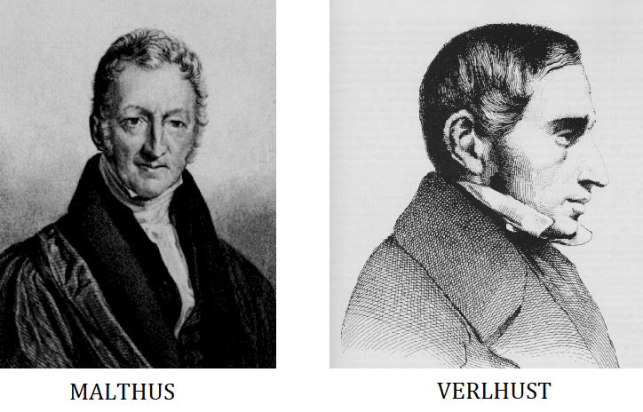
In 1840, Verlhust proposed a more suitable growth model based on the assumption that the growth rate $r$ is not a constant but is an affine function of the population size $y$:
\[y'(t) = \big(n(y) - m(y)\big) y(t)\]Verlhust notably starts from the hypothesis that the more the size of a population increases, the more its birth rate $n$ decreases and the more its death rate $m$ increases. Starting from this hypothesis and applying some clever algebraic manipulations, we can show that the previous differential equation can be rewritten in the form:
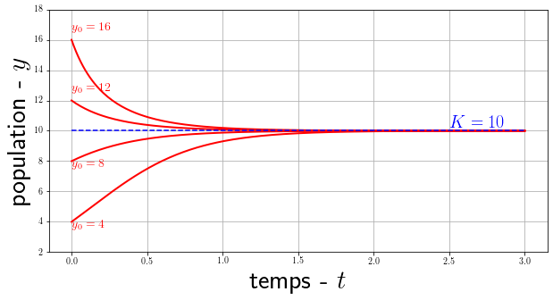
\[y'(t) = r y(t) \left(1 - \frac{y(t)}{K}\right)\]with $K$ a constant called accommodation capacity. We can analytically solve this equation with the initial condition $y(t=0)=y_0$, we obtain the logistic solution:
\[y(t) = \frac{K}{1+\left(\frac{K}{y_0}-1\right)e^{-rt}}\]
Detailed solution of the logistic differential equation by variable separation
$$ \begin{align*} \int_{y_0}^{y(t)} \frac{1}{y(1-y/K)}dy &= \int_0^t r \ d\tau \\ \int_{y_0}^{y(t)} \frac{K}{y(K-y)}dy &= \int_0^t r \ d\tau \\ \int_{y_0}^{y(t)} \frac{1}{y}dy + \int_{y_0}^{y(t)} \frac{1}{K-1}dy &= \int_0^t r \ d\tau \\ \ln \left| \frac{y(t)}{y_0} \right| - \ln \left| \frac{K-y(t)}{K-y_0} \right| &= r \ t \\ \ln \left( \frac{y(t)\big(K-y_0\big)}{y_0\big(K-y(t)\big)} \right) &= r \ t \\ \frac{y(t)}{K-y(t)} &= \frac{y_0}{K-y_0}e^{rt} \\ y(t)\left(1+\frac{y_0}{K-y_0}e^{rt} \right) &= \frac{K y_0 e^{rt}}{K-y_0} \\ y(t) &= \frac{Ky_0e^{rt}}{K-y_0+y_0e^{rt}} \\ y(t) &= \frac{K y_0}{(K-y_0)e^{-rt}+y_0} \\ \end{align*} \\ \square $$Note that $ \lim\limits_{t\to\infty} y(t) = K $. This means that regardless of the size of the initial population $y_0$, the population will always end up tending towards $K$ the carrying capacity that is often qualified as the maximum number of individuals that the environment can accommodate (according to space, resources, etc.). This so-called logistic function introduced for the first time by Verlhulst to model the growth of populations will subsequently find many applications in various fields such as economics, chemistry, statistics and more recently artificial neural networks.
Lotka-Volterra Model
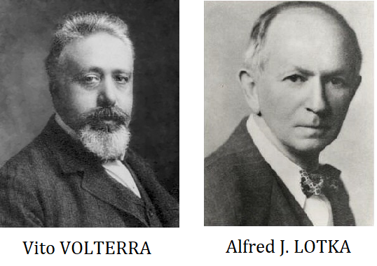
Lotka-Volterra models are systems of simple equations that appeared at the beginning of the 20th century. They bear the name of two mathematicians who published simultaneously but independently on the subject: Volterra, in 1926, to model the populations of sardines and their predators and Lotka, in 1924, in his book Elements of Physical Biology. Unlike the Verlhust model, which focuses on a single population, the Lotka-Volterra models model the interactions between several species, each having an impact on the development of the other.
Prey-predator
The prey-predator model of Lotka-Volterra has made it possible to explain data collected from certain populations of animals such as the lynx and hare as well as the wolf and the elk in the United States. It represents the evolution of the number of prey $x$ and predators $y$ over time $t$ according to the following model:
\[\left\{ \begin{array}{ccc} x'(t) = x(t)\ \big(\alpha - \beta y(t)\big) \\ y'(t) = y(t)\ \big( \delta x(t) - \gamma\big) \end{array} \right.\]with the parameters $\alpha$ and $\delta$ are the reproduction rates of prey and predators respectively and $\beta$ and $\gamma$ are the mortality rates of prey and predators respectively.
Note: We speak of an autonomous system: the time $t$ does not appear explicitly in the equations.
If we develop each of the equations, we can more easily give an interpretation. For prey, we have on the one hand the term $\alpha x(t)$ which models exponential growth with an unlimited source of food and on the other hand $- \beta x(t) y(t)$ which represents predation proportional to the frequency of encounter between predators and prey. The equation for predators is very similar to that for prey, $\delta x(t)y(t)$ is the growth of predators proportional to the amount of food available (the prey) and $- \gamma y(t) $ represents the natural death of predators.
We can calculate the equilibria of this system of differential equations and also deduce a behavior from it, but the solutions do not have a simple analytical expression. Nevertheless, it is possible to compute an approximate solution numerically (more details in the next section).
# define ODE function to resolve
r, c, m, b = 3, 4, 1, 2
def prey_predator(XY, t=0):
    dX = r*XY[0] - c*XY[0]*XY[1]
    dY = b*XY[0]*XY[1] - m*XY[1]
    return [dX, dY]
# discretization
T0   = 0
Tmax = 12
n    = 200
T    = np.linspace(T0, Tmax, n)
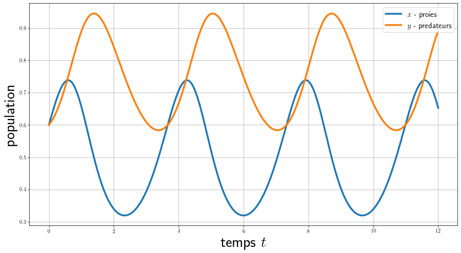
Here we calculate the evolution of the 2 populations as a function of time for a fixed initial condition, we see that they have a periodic behavior and a phase shift.
# TEMPORAL DYNAMIC
X0 = [1,1]
solution = integrate.odeint(prey_predator, X0, T) # use scipy solver
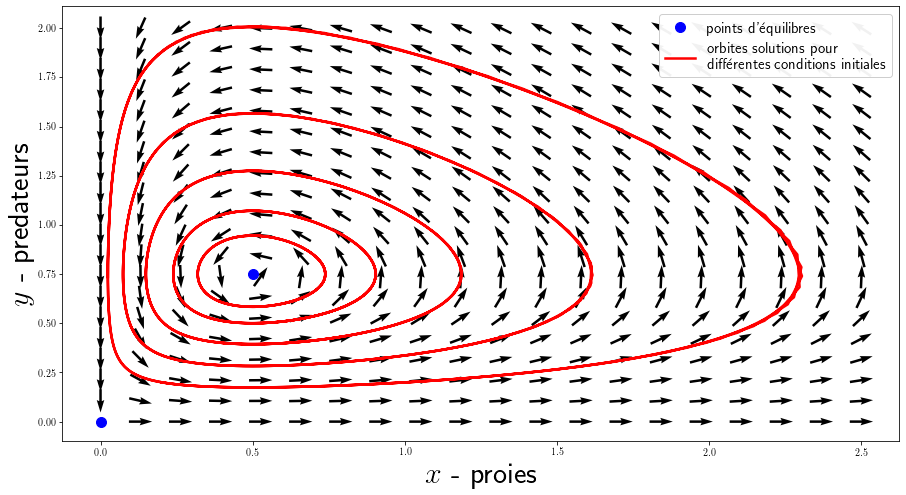
Here, we calculate several solutions for different initial conditions that we display in phase space (time does not appear). You can also display the vector field generated by the system of equations with plt.quiver() for a grid of values.
# PHASES SPACE
# some trajectories
orbits = []
for i in range(5):
    X0    = [0.2+i*0.1, 0.2+i*0.1]
    orbit = integrate.odeint(prey_predator, X0, T)
    orbits.append(orbit)
# vector field
x, y             = np.linspace(0, 2.5, 20), np.linspace(0, 2, 20)
X_grid, Y_grid   = np.meshgrid(x, y)
DX_grid, DY_grid = prey_predator([X_grid, Y_grid])
N                = np.sqrt(DX_grid ** 2 + DY_grid ** 2)
N[N==0]          = 1
DX_grid, DY_grid = DX_grid/N, DY_grid/N
Warning: The units of the simulations do not reflect reality, populations must be large enough for the modeling to be correct.
In the model used, predators thrive when prey is plentiful, but eventually exhaust their resources and decline. When the predator population has diminished enough, the prey taking advantage of the respite reproduce and their population increases again. This dynamic continues in a cycle of growth and decline. There are 2 equilibria: the point $(0,0)$ is an unstable saddle point which shows that the extinction of the 2 species is in fact almost impossible to obtain and the point $(\frac{\gamma}{\delta }, \frac{\alpha}{\beta})$ is a stable center, the populations oscillate around this state.
Note: This modeling remains quite simple, a large number of variants exist. We can add terms for the disappearance of the 2 species (due to fishing, hunting, pesticides, etc.), take into account the carrying capacity of the environment by using a logistical term.
Competition
The Lotka-Volterra competition model is a variant of the predation model where the 2 species do not have a hierarchy of prey and predators but are in competition with each other. Moreover, the basic dynamic is no longer a simple exponential growth but a logistic one (with the parameters $r_i$ and $K_i$):
\[\left\{ \begin{array}{ccc} x_1'(t) = r_1x_1(t)\left(1- \frac{x_1(t)+\alpha_{12}x_2(t)}{K_1}\right) \\ x_2'(t) = r_2x_2(t)\left(1- \frac{x_2(t)+\alpha_{21}x_1(t)}{K_2}\right) \end{array} \right.\]with $\alpha_{12}$ the effect of species 2 on the population of species 1 and conversely $\alpha_{21}$ the effect of species 2 on species 1. For example, for the species 1 equation, the coefficient $\alpha_{12}$ is multiplied by the population size $x_2$. When $\alpha_{12} < 1$ then the effect of species 2 on species 1 is smaller than the effect of species 1 on its own members. And conversely, when $\alpha_{12} > 1$, the effect of species 2 on species 1 is greater than the effect of species 1 on its own members.

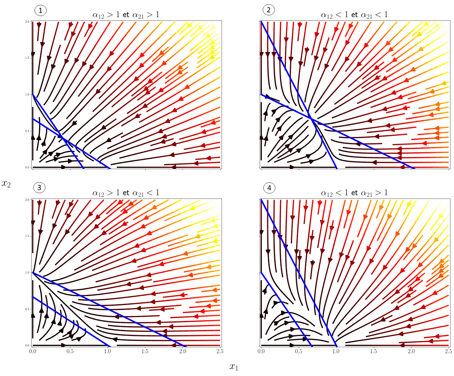
To understand the predictions of the models in more detail, it is useful to plot the phase space diagrams $(x_1,x_2)$ as before. We can distinguish 4 scenarios according to the values of the competition coefficients, I display below the vector fields of these scenarios with plt.streamplot() as well as the isoclines, the curves for which \(x_1'(t) =0\) or \(x_2'(t)=0\):
# define ODE to resolve
r1, K1 = 3, 1
r2, K2 = 3, 1
def competition(X1X2, a1, a2):
    dX1 = r1*X1X2[0] * (1-(X1X2[0]+a1*X1X2[1])/K1)
    dX2 = r2*X1X2[1] * (1-(X1X2[1]+a2*X1X2[0])/K2)
    return [dX1, dX2]
# compute derivatives for each scenario
N = 20
x, y = np.linspace(0, 2.5, N), np.linspace(0, 2, N)
X_grid, Y_grid = np.meshgrid(x, y)
DX_grid, DY_grid = np.zeros((4,N,N)), np.zeros((4,N,N))
coeffs = np.array([[1.5,1.5],[0.5,0.5],[1.5,0.5],[0.5,1.5]])
for k,(a1,a2) in enumerate(coeffs):
    DX_grid[k,:], DY_grid[k,:] = competition([X_grid, Y_grid], a1, a2)
In the end, the 4 possible behaviors depending on $\alpha_{12}$ and $\alpha_{21}$ are the following:
- Competitive exclusion of one of the two species depending on the initial conditions.
- Stable coexistence of the two species.
- Competitive exclusion of species 1 by species 2.
- Competitive exclusion of species 2 by species 1.
The stable coexistence of the 2 species is only possible if $\alpha_{12} < 1$ and $\alpha_{21} < 1$, i.e. interspecific competition must be weaker than intraspecific competition.
Numerical method for ODEs
This section is a little bit apart from the real subject of this post since I introduce numerical methods to solve differential equations. Indeed, it is possible to deduce many properties of an ODE system based on mathematical theorems for the theory of dynamical systems (Lyapunov method, LaSalle invariance, Poincaré-Bendixon theorem …) but only a restricted number of differential equations admit an analytical solution. In practice, we often prefer to have a method that computes an approximate solution of the problem at any time $t$. We consider the problem \(y'(t) = f\big(t,y(t)\big)\) with $y(t_0)=y_0$. The idea of numerical methods is to solve the problem on a discrete set of points $(t_n,y_n)$ with $h_n=t_{n+1}-t_n$, a fixed time step.
Euler
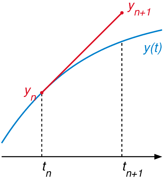 Euler’s method is the most basic numerical method for ODE, it uses the differential equation to calculate the slope of the tangent at any point on the solution curve. The solution is approached starting from the known initial point $y_0$ for which the tangent is calculated, then a time step is taken along this tangent, a new point $y_1$ is then obtained. The idea is to repeat this process, for a time step from $t_n$ to $t_{n+1}$ we can write it as $y_{n+1} = y_n + hf(t_n,y_n)$ .
This method is very simple to set up, for example in python:
def Euler_method(f, y0, t):
    y = np.zeros((len(t), len(y0)))
    y[0,:] = y0
    for i in range(slow(t)-1):
        y[i+1] = y[i] + h*f(y[i], t[i])
    return y
Runge Kutta
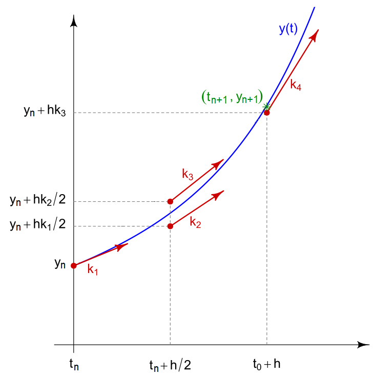 Runge-Kutta methods are a family of methods, the best known is that of order 4 It is more precise than the Euler method by making a weighted average of 4 terms corresponding to different slopes of the curve in the fixed time interval. It is defined by:
with:
- $k_1=f(t_n,y_n)$
- $k_2=f(t_n+h/2,y_n+hk_1/2)$
- $k_3=f(t_n+h/2,y_n+hk_2/2)$
- $k_4=f(t_n,y_n+hk_3)$
def RungeKutta4_method(f, y0, t):
    y = np.zeros((len(t), len(y0)))
    y[0] = y0
    for i in range(len(t)-1):
        k1 = f(y[i], t[i])
        k2 = f(y[i]+k1*h/2, t[i]+h/2)
        k3 = f(y[i]+k2*h/2, t[i]+h/2)
        k4 = f(y[i]+k3*h, t[i]+h)
        y[i+1] = y[i] + (h/6) * (k1 + 2*k2 + 2*k3 + k4)
    return y
Example
To verify the behavior of these methods, I chose to test them on a well-known model of physics: the harmonic oscillator. In its simplest form, we can calculate exactly the solution of the problem and therefore compare our approximate resolution methods. The problem can be written:
\[\left\{ \begin{array}{ccc} y''(t) + y(t) = 0 \\ y(0) = y_0 \end{array} \right.\]and admits for solution $ y(t) = y_0 \cos(t) $.
# initial condition
y0 = [2, 0]
# discretization
t = np.linspace(0.5*pi, 100)
h = t[1] - t[0]
# ODE wording
defproblem(y, t):
    return np.array([y[1], -y[0]])
# analytics solution
def exact_solution(t):
    return y0[0]*np.cos(t)
y_exact = exact_solution(t)
y_euler = Euler_method(problem, y0, t)[:, 0]
y_rk4 = RungeKutta4_method(problem, y0, t)[:, 0]
As expected the Runge-Kutta method is much more accurate than the Euler method (but slower). The error of the numerical methods decreases according to the size of the time step $h$ but the smaller $h$ is, the longer the calculation time. In theory, to analyze numerical methods, we base ourselves on 3 criteria:
- the convergence which guarantees that the approximate solution is close to the real solution.
- the order which quantifies the quality of the approximation for an iteration.
- the stability which judges the behavior of the error.
In practice: In the previous problems , I use the integrate.odeint(f, y0, t) function from scipy which is a more advanced ODE solver that uses the method of Adams–Bashforth
![]()
![]()
![]()
![]()
-
The term ordinary is used as opposed to the term partial differential equation (or partial differential equation) where the unknown function(s) may depend on more than one variable. ↩
Laisser un commentaire