Fractal Object: Dimension, Self-Similarity, Infinity

They are present in tropical forests, at the forefront of medical research, in films and everywhere where wireless communication reigns. This mystery of nature has finally been unraveled. “Damn, but it’s of course !”. Perhaps you have never heard of these strange shapes, yet they are everywhere around you. Their name: fractals.

ARTE report – in search of the hidden dimension

Introduction

As you will have understood if you watched the excellent ARTE documentary presented above, fractals are infinitely fragmented geometric objects which have the particularity of presenting similar structures at all scales. This type of geometry makes it possible to model with simple recursive formulas infinitely complex figures but also to describe natural phenomena (patterns of snowflakes, path taken by lightning, shape of a cabbage of romanesco, structure of lungs …) and to find applications in technological fields (antennas, transistors, graphic generation of landscapes…).

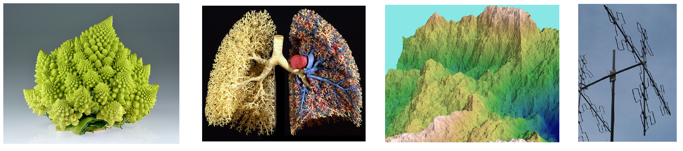
Note: Fractals found in nature are finite approximations of real mathematical objects.

Fractals are notably characterized by the counter-intuitive notion of non-integer dimension. Indeed, we can define a general scaling rule that links the measure $N$, a scale factor $\varepsilon$ and the dimension $D$:

\[N = \varepsilon^{-D}\]

For example, for a usual geometric figure like the square, its dimension is $D=2$ and if we subdivide it into $3$ its area is $N=9$, we have $9=\frac{1}{3} ^{-2}$. We can apply this same reasoning for a cube or even a line.

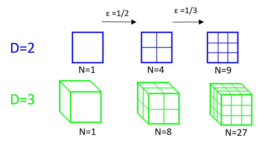
Now, we seek to find the dimension of a simple fractal figure. The above formula gives us: \(D = -\frac{\log N}{\log \varepsilon}\)

If we are interested in a figure such as the Von Koch curve which consists, from a segment, of recursively constructing equilateral triangles on each sub-segment (see animation below). By counting the segments at each new scaling, we understand that the length of the Koch curve is multiplied by $4$ for each scaling $\varepsilon=\frac{1}{3}$ (we divides the segments by 3). We therefore find that its dimension is $D = \frac{\log 4}{\log 3} \approx 1.26$. It is not a simple one-dimensional curve, nor a surface but something “in between”.

Note: The approach presented above is conceptual. A rigorous and definite definition for any set is the Hausdorff dimension. It is not easy to implement…

We can differentiate 3 main categories of fractal:

• systems of iterated functions. They have a fixed geometric rule like Von Koch’s snowflake, Sierpinski’s carpet, Peano’s curve.
• random fractals. They are generated by a stochastic process as in nature or fractal landscapes.
• the sets defined by a recurrence relation at each point of a space. We can cite the set of Julia, Mandelbrot, Lyapunov. They are sometimes called Escape-time fractals.

Julia’s set

The Julia set associated with a fixed complex number $c$ is the set of initial values ​​$z_0$ for which the following sequence is bounded:

\[\left\{ \begin{array}{ll} z_0 \in \mathbb{C} \\ z_{n+1} = z_n^2 + c \end{array} \right.\]

To generate a Julia set by computer, the idea is to discretize the space in a fixed interval to have a finite number of value $z_0$ for which we will test the convergence of the sequence.

# INITIALIZATION
# value of c fixed
c_reel, c_imag = 0.3, 0.5 
# interval limit
x_min, x_max = -1, 1
y_min, y_max = -1, 1
# discretization
size = 5000 
x_step = (x_max - x_min)/size
y_step = (y_max - y_min)/size
M = np.zeros((size,size))

To be able to work with complex numbers, I chose to decompose the real part z_real and the imaginary part z_image. Then, we test the convergence for a given point by looking if we have not exceeded a finite number of iterations n_iter < itermax. We can also, in addition, check that the sequence $(z_n)$ is divergent if its modulus is strictly greater than $2$, z_reel**2 + z_imag**2 < 4 (cf demonstration). Finally, we can fill a matrix M with $0$ or $1$ according to the convergence test. But, for a more aesthetic final visual rendering, we can also fill the M matrix according to the estimated convergence rate with n_iter/itermax.

# LOOP ON ALL PIXEL = COMPLEX PLANE
for i in (range(size)):
    for j in range(size):
        n_iter = 0
        # convert pixel position to a complex number
        z_reel = i * x_step + x_min
        z_imag = j * y_step + y_min
        # update sequence until convergence
        while (z_reel**2 + z_imag**2 < 4) and (n_iter < itermax):
            z_reel, z_imag = z_reel**2 - z_imag**2 + c_reel, 2*z_imag*z_reel + c_imag
            n_iter = n_iter + 1
        # color image according to convergence rate
        M[j,i] = 255*n_iter/itermax

Tip: In python, we could have directly used the complex() function to have a complex object. In this case, the z_reel and z_imag variables would be useless and one could directly retrieve the absolute value and square a single complex variable z.

Finally, we can generate Julia sets for different fixed values ​​of $c$ and to change the visual we can have fun testing different colormap. Below are some results I generated.

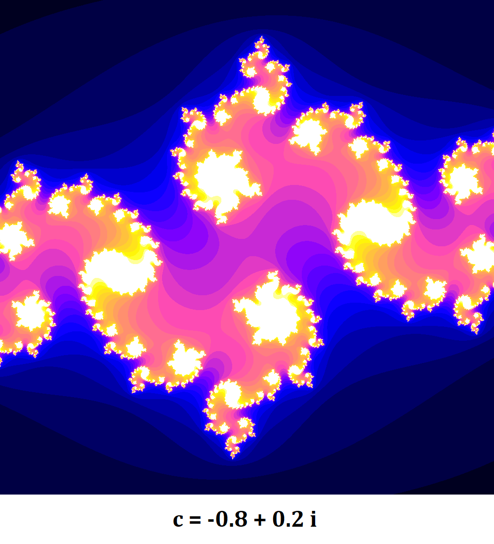
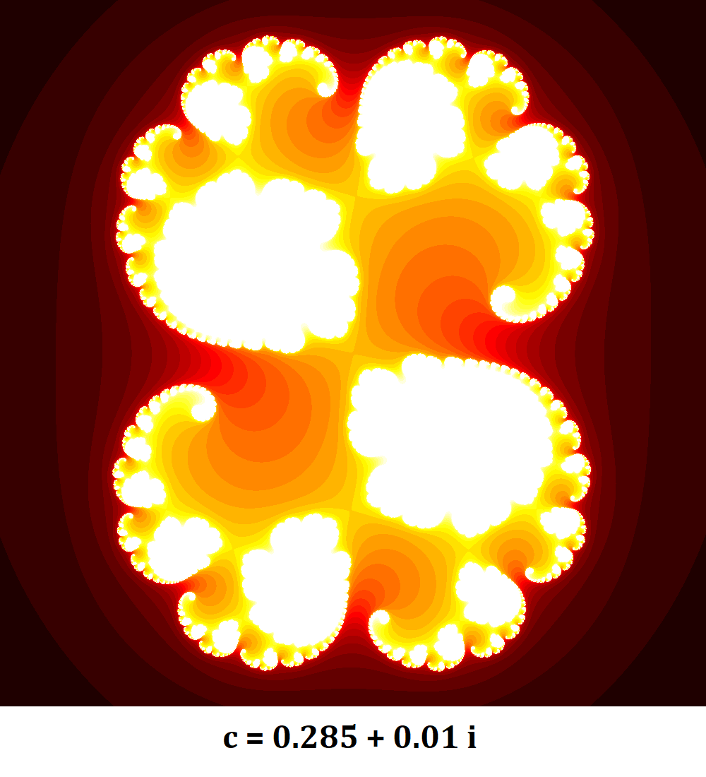
Note that the figures obtained vary greatly depending on the value of the complex $c$ chosen. In fact, one can generate the sets of julia for a sequence of consecutive complexes to see how the figures evolve and make an animation of them.

Mandelbrot set

The Mandelbrot set is strongly related to the Julia sets, indeed we can define the Mandelbrot set $M$ as the set of complexes $c$ for which the corresponding Julia set $J_c$ is **connected **, that is to say, it is made of a single piece. We can say that the Mandelbrot set represents a map of Julia sets. And, contrary to the name it bears, it was the mathematicians Julia and Fatou who discovered it and who showed that the previous definition is equivalent to the set of points $c$ of the complex plane $\mathbb{C }$ for which the following sequence is bounded:

\[\left\{ \begin{array}{ll} z_0 = 0 \\ z_{n+1} = z_n^2 + c \end{array} \right.\]

This definition is very similar to that of the Julia set except that we are interested in the variable $c$. In the previous code, the line z_reel = i * x_step + x_min should be modified by c_reel = i * x_step + x_min and set z_reel = 0 (same for the imaginary part). We get the following figure:

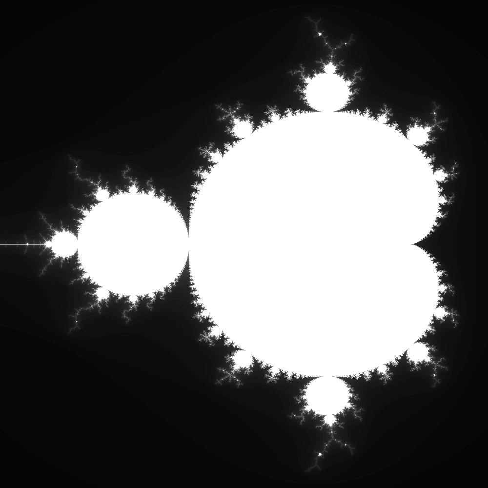
Note: Benoît Mandelbrot is the founder of fractal theory with his article “How Long Is the Coast of Britain? Statistical Self-Similarity and Fractional Dimension” in 1967. It is also he who obtained for the first time, a computer visualization of this set.

Software

Fractal generation is not an easy task: many parameters can be taken into account and calculation times are often long. In the figures that I generated, we do not see at first sight the self-similar character of fractals, it would be necessary to change scale by zooming in deeper and deeper on a point of the plane.

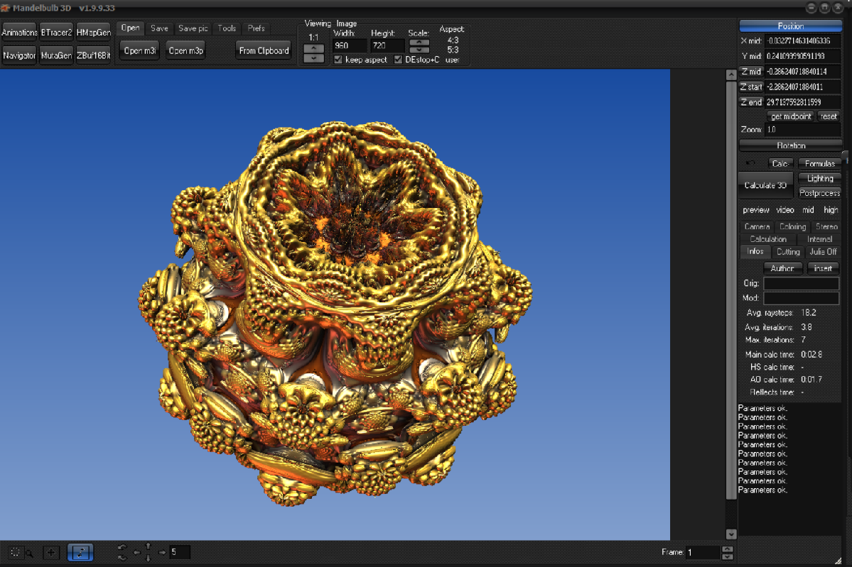
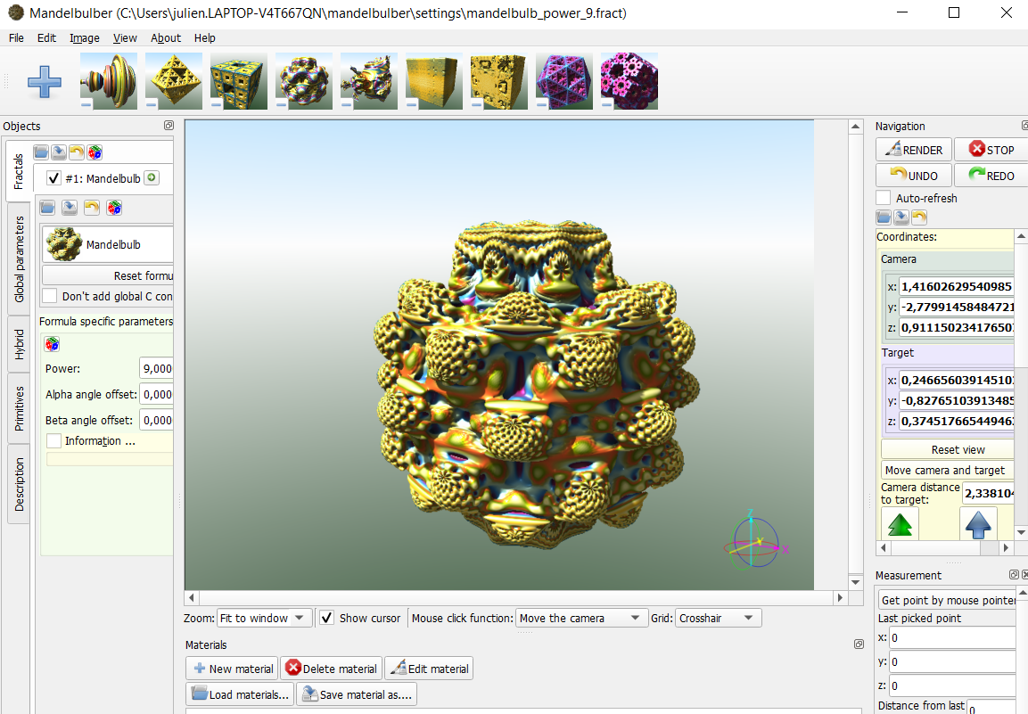
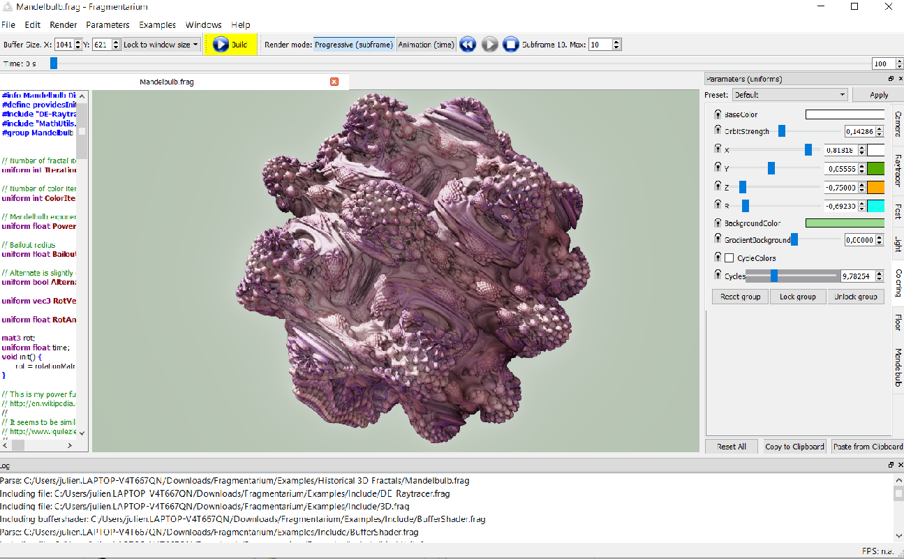
There are many free fractal generator software available. They are often optimized for multi-processing or GPU computing, have a graphical interface to manage the many parameters and are sometimes capable of creating 3D objects (like the 3 displayed below). A fairly comprehensive list is available here.

Mandelbul3D	Mandelbuler	Fragmentarium

And for those who do not want to complicate themselves and just let themselves be carried away by the psychadelic geometry of fractals without effort, you can find people on the internet who have already done the work for you. There are a slew of videos on youtube such as The Hardest Trip - Mandelbrot Fractal Zoom which zooms in for 2h30 on a specific point of the complex plane.

---